3.1 Introduction
The dimension of Sustainability within the New European Bauhaus (NEB) paradigm identifies the environmental and economic perspectives as two main drivers to promote a holistic approach for the design or renovation of buildings and living spaces that are not only ecologically responsible, but also financially viable in the long term. This approach encourages the development of innovative solutions that minimise environmental impacts, while also generating economic value, thus fostering a symbiotic relationship between ecological stewardship and economic prosperity.
The environmental perspective of the sustainability dimension needs to address issues related to energy, greenhouse gas (GHG) emissions, and other non-energy related environmental impacts from the built environment, as follows:
Energy – The European Union (EU) building stock, including both the residential and service segments, constitutes the most energy demanding sector in the 27 European Union Member States (EU-27), reaching 391.2 million tonnes of oil equivalent (Mtoe) in 2021, corresponding to 44 % of the EU total final energy consumption (European Commission, 2023a). The use of fossil fuels for direct combustion represents 43 % of the final energy consumption in the EU buildings, followed by electricity at 29 % and renewables at 17 %. The operation of buildings is responsible for significant environmental impacts due to the indirect emissions associated with the generation of electricity, since 58 % of the final electricity consumption is used in EU buildings. The gross electricity generation in the EU-27 depends on over 37 % of fossil fuels (i.e. 20 % natural and manufactured gas, 15 % solid fuels and 2 % oil), 38 % renewables (i.e. 13 % wind, 13 % hydro, 6 % solar, 4 % solid biofuels, and 2 % biogases) and 25 % nuclear (Energy datasheets 2024).
Accordingly, the 2024 recast Energy Performance of Buildings Directive (EPBD) (Directive 2024/1275) requires very high energy performance buildings with zero or minimum direct and indirect use of fossil fuels. Specifically, the minimum building code requirements across the EU-27 for new buildings and major renovations are the nearly zero-energy buildings (NZEBs) that will evolve towards further enhanced zero-emission buildings requirements, i.e. require zero or a very low amount of energy, producing zero on-site emissions.
NZEBs shall exhibit nearly-zero or very low energy demand that should be covered to a very significant extent by renewable energy sources (RES), combined heat and power (CHP) generation or efficient district heating and cooling, whereas zero-emission buildings require zero or a very low amount of energy and produce zero on-site carbon emissions from fossil fuels. The 2024 recast EPBD (Directive 2024/1275) set that each EU-27 Member State shall establish a trajectory for the progressive renovation of its residential building stock ensuring the reduction of the average primary energy use of residential buildings by at least 16 % by 2030 and at least 20-22 % by 2035, compared to 2020. Furthermore, Member States shall ensure that at least 55 % of the decrease in the average primary energy use is achieved through the renovation of the 43 % worst-performing residential buildings (Directive 2024/1275). New buildings will have to be solar-ready, meaning they have to be fit to host the installation of rooftop photovoltaic or solar thermal installations, thus leading solar energy systems to become part of minimum requirements for all new public and non-residential and residential buildings. For existing public and non-residential buildings, the installation of solar systems shall be gradually ensured by 2027-2030, depending on the useful floor area of buildings, if the installation is technically suitable, and economically and functionally feasible.
- GHG emissions – The GHG emissions associated with the building sector include direct emissions from onsite combustion for heating and indirect emissions from power plants to generate electricity using solid, liquid, and gas fossil fuels, as well as gas flaring. In 2021 the direct GHG emissions from fuel combustion amounted to 17 % of the total emissions in the EU-27, mainly dominated by carbon dioxide (CO2) emissions from fossil fuels (EEA, 2023). However, the largest key category for the GHG emissions in the EU-27 is from public electricity and heat production that annually contributes to about 20 % of the total GHG emissions (European Commission, 2023). Collectively, the operation of buildings contributes to about 25 % of the total GHG emissions in the EU-27. Accounting for the emissions associated with the construction industry will also add another 10 % from manufacturing building products and materials, which is associated with the embodied carbon. The recast EPBD (Directive 2024/1275) set a new minimum requirement for new buildings which shall be zero emissions buildings across the EU-27 as of 1 January 2028 for buildings owned by public bodies, and as of 1 January 2030 for all other new buildings. New buildings shall require zero or a very low amount of energy, producing zero on-site carbon emissions from fossil fuels and produce zero or a very low amount of operational greenhouse gas emissions, determined according to the Annexes in recast EPBD (Directive 2024/1275). Furthermore, deep renovation should transform existing buildings into zero-emission buildings after 2030.
The EU transport sector is responsible for nearly a quarter of the EU total GHG emissions that has been increasing since 1990 (European Commission, 2023a). Projections indicate that domestic transport emissions will only drop below their 1990 level in 2029. Road transport exhibits the highest proportion of GHG emissions, reaching 73 % of the total amount of the EU GHG emissions due to transport, also including international aviation and international navigation, in 2022 (European Commission, 2024). The European Green Deal (COM, 2019/640) calls for a 90 % reduction in GHG emissions from transport to meet the overarching goal for the EU of being the first continent with a climate-neutral economy by 2050, while also working towards a zero-pollution ambition.
- Other non-energy related environmental impacts - Beyond energy consumption and GHG emissions, the built environment also generates significant impacts related to air, water, and raw materials.
Indoor air quality in buildings is very important as it can impact human health, since Europeans spend more than 90 % of their time inside buildings. Studies reveal that indoor air quality may directly threaten the occupants’ health and, in some cases, may also be twice as polluting as outdoor air (European Commission, 2003). As a result, building occupants are exposed to hundreds of volatile components and some of them are toxic, mutagenic or carcinogenic. National regulations for indoor pollutants, such as carbon dioxide (CO2), formaldehyde (CH2O), particulate matter (PM), nitrogen dioxide (NO2), carbon monoxide (CO), and radon (Rn) define acceptable levels in relation to human well-being inside buildings and building energy performance (Dimitropoulou et al., 2023).
Water is a vital natural resource, thus its management and consumption are considered major concerns of the environmental protection at EU level, according to the Water Framework Directive (Directive 2000/60/EC). The building sector is responsible for a significant pressure on this natural resource leading to a major concern for its handling, since about 21 % of all water abstracted in the EU is used for public supply, the majority of which is used in buildings (Donatello et al., 2021a). Furthermore, in the EU households the use of water from public supply averages around 40-50 m3 per inhabitant (Eurostat, 2023a).
The built environment accounts for half of all extracted raw materials and produce vast quantities of construction and demolition waste (CDW), thus being responsible for over 35 % of all waste generated in the EU (COM 2020/98). A change of direction based on the increase of material efficiency has led the EU to promote circularity principles and design for deconstruction practices to recover reusable materials from demolished buildings, also avoiding GHG emissions due to the production of new materials. In addition low-carbon building materials and energy-efficient construction techniques play a pivotal role in reducing the carbon footprint of the construction sector. The ultimate goal of circular construction is to eliminate waste from the construction value chain and reduce the reliance of the construction sector on finite resources.
The economic perspective of sustainability for projects in line with the NEB initiative (COM 2021/573) should follow the three levels of ambition introduced in the Compass (European Commission, 2022): (i) to repurpose, (ii) to close the loop and (iii) to regenerate. The economic perspective of sustainability addresses two main aspects: (i) a more efficient use of scarce resources and the use of less money in a more effective way, and (ii) the investigation and collection of diverse potential sources of existing public funding and available private funding to support projects. Hence, projects that are consistent with the eligible criteria of existing funding and/or prospect innovative and integrated ways to collect private financing should be favoured, with the secondary effect of reducing the amount of public expense.Specifically, the growing interest of the private sector in sustainable finance, which relies on non-financial factors, i.e. environmental, social, and governance (ESG) criteria, should be used to advertise and offer coherent development opportunities. This approach becomes potentially more participatory, promoting the interaction across institutional levels and the involvement of private stakeholders that also include single citizens or local groups interested in crowdfunding campaigns.
In this context, three domains define the economic perspective of building and living space projects in line with the NEB concept:
- Greening the public sector in terms of its economic involvement in the sustainability of the built environment – Public investment in buildings and living spaces aims to transform places or the functions provided to the community, thus creating value for people. In this sense, ‘greening of the public sector’ aims to emphasise the role of public sector as a pioneer and demonstrator.
- Greening the private and financial sector in terms of its economic involvement in the sustainability of the built environment – The promotion of the NEB vision requires the private and financial sector to be as innovative and forward-thinking as the designers and architects of projects. The financial sector can play a pivotal role in materialising the NEB vision by developing specialised financial products, navigating the dynamic regulatory framework, embracing long-term investment strategies, leveraging technology, building capacities, engaging in international collaborations, and prioritising community engagement.
Promote circular economy (CE) – Circular economy is an emerging approach to resource management focusing on the design of processes agenda and encouraging more upstream solutions and interventions towards a systemic change. CE is regenerative by design, built on the principles of eliminating waste and pollution, keeping products and materials in use, and regenerating natural systems. In 2015, the European Commission introduced its first circular economy action plan (COM, 2015), leading to the adoption of the new version of this action plan in 2020 (COM, 2020a) as one of the main blocks of the Euroepan Green Deal. The NEB initiative provides Europe with the opportunity to demonstrate the potential of the circular economy that moves from technicalities and resource economics to achieve a circular society, leading to adeep cultural resonance. CE leads to several advantages for the economy and its functions. Many economic benefits and opportunities due to CE are long-term and indirect and require significant investment. Hence, long-term benefits are a key-point to consider, as well as short-term incentives, to drive the change. In this context, policies that create more immediate financial incentives for businesses may facilitate the development of innovative new business models and enable the efficient flow of reused and recycled materials across global value chains. According to the United Nations Environmental Programme (UNEP), in 2050, the global economy will benefit by USD 2 trillion a year from more effective resource management (Ekins et al., 2017) since the cost of raw materials will decrease substantially while promoting employment and innovation. Although the attention for the circular economy is increasing, the extraction and prices of primary raw materials are still rising and the global circularity rate results into a steady decline, passing from only 9.1 % of all raw materials fully recycled in 2018 to 7.2 % in 2023 (CEF, 2024). A theoretical full circular economy corresponds to the recycling of 100 % of generated waste in secondary raw materials so that no new virgin raw materials are needed. However, this scenario can be achieved in a very long time, as it is still needed to develop effective methods to fully recycle materials that are currently used in products (Fellner et al., 2017).
3.2 Assessment targets to achieve
Sustainability concerns are addressed by assessing their status or progress towards nine targets related to both environmental and economic perspectives. The targets considered within the environmental perspective mainly refer to energy (e.g. direct operational energy demand, and use of renewables), greenhouse gas emissions due to operational-embodied energy and sustainable mobility, and non-energy related environmental impacts to air, water, and the use of materials along with construction and demolition-related waste. The targets reflected within the economic perspective regard the role of the economic involvement of the public sector, the private and financial sector, and the promotion of circular economy.
3.2.1 Minimise fossil fuel use
Energy efficiency first principle (Directive 2023/1791) is the main guiding principle, complementing relevant EU objectives in sustainability, climate neutrality and green growth, becoming particularly significant in the construction sector to achieve buildings that exhibit a very low energy use from conventional or renewable energy sources. Hence, it is essential to minimise the primary energy consumption of buildings and maximise the use of renewable energy sources in line with the provisions of the recent recast EPBD (Directive 2024/1275).
In this context, the use of fossil fuels needs to be extensively reduced according to the following three objectives:
- Minimise the primary energy demand of buildings.
- Minimise the electricity peak demand for building operations, resulting into an essential goal considering the current electrification era of the building sector.
- Optimise the smart readiness (SR) capacity of buildings to sense, interpret, communicate, and actively respond in an efficient way to changing conditions related to the operation of technical building systems, the external environment (including energy grids) and the demand from building occupants. At a larger scale of a neighbourhood or a city, the smart readiness issues are addressed by smart meters to automatically monitor and adjust energy flows in response to changes in energy supply and demand, and possibly cost.
The primary energy demand is part of the definition of a Nearly Zero-Energy Building (NZEB), as introduced in the 2010 recast EPBD (Directive 2010/31) and confirmed in the recent revised EPBD (Directive 2024/1275), to assess the energy performance of a building during its use stage. The energy performance of a building is also referred to as annual primary energy consumption, defined as any kind of extraction of energy products from natural sources to a usable form. The exploitable natural resources include coal, crude oil, natural gas, etc., while the transformation of energy from one form to another, such as electricity or heat generated by thermal power plants, is not included in the primary energy production. Energy and climate targets set in the EU policies and legislative instruments are commonly articulated around the concept of primary and final energy consumption and emissions. The commitment to improve energy efficiency by 20 % by 2020 and the new binding energy efficiency target of reducing the EU energy consumption of at least 11.7 % by 2030, compared to the 2020 EU reference scenario projections for 2030 (Directive 2023/1791), represent examples in this direction, as the need to improve the EU energy efficiency is generally expressed in primary and final energy consumption. Indeed, this 2030 ambitious target translates into a EU primary energy consumption target of 992.5 Mtoe and a final energy consumption target of 763 Mtoe in 2030 (Figure 5), corresponding to a reduction of 40.5 % and 38 % of primary and final energy consumption, respectively (compared to the 2007 EU reference scenario projections for 2030). The construction and renovation of buildings are recognised as some of the sectors with the greatest potential for energy savings, thereby using energy more efficiently, thus the EU established the requirement of NZEB buildings since 2020 towards zero-emissions buildings starting from 2028-2030 (Directive 2024/1275). However, the NZEB and zero-emission building requirements do not usually apply to the following categories of buildings: (i) buildings officially protected as part of a designated environment or because of their special architectural or historical merit, (ii) buildings used as places of worship and for religious activities, (iii) temporary buildings with a time of use of two years or less, (iv) residential buildings which are used or intended to be used for either less than four months of the year, (v) stand-alone buildings with a total useful floor area of less than 50 m2 and (vi) buildings owned by the armed forces or central government and serving national defence purposes.
Figure 5. Primary and final energy consumption from 2005 to 2022 in EU-27
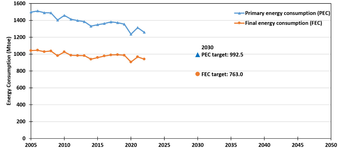
Source: Adapted from European Environment Agency (EEA, 2024a); data from Eurostat, 2022.
The electricity peak demand is emerging to a major issue in the era of building electrification and represents the maximum amount of electricity demand required for building operation on a yearly basis. Advanced measurement technologies, demand response and smart grids facilitate building monitoring to manage peak demand. This contributes to grid stability and reduces environmental impacts by decreasing reliance on fossil fuels during peak periods. Energy-efficient buildings, demand response programs, energy storage systems, and the integration of renewable energies are just some of the strategies used to mitigate peak demand in buildings. The use of automation systems, occupant education, time-based scheduling, and the adoption of energy-efficient lighting and electrical appliances further contribute to the electricity peak demand reduction, leading to lower energy costs and contributing to greater sustainability and a more comfortable indoor environment.
The smart readiness of a building refers to its ability to use information technologies and electronic systems to adapt the operation of buildings to the needs of the occupants and the energy grid, as well as to improve the overall in-use energy performance of buildings, thus achieving a more energy-efficient, environmentally friendly, healthy, and comfortable indoor, in line with the recent EPBD recast (Directive 2024/1275). Smart readiness raises awareness of the benefits of smarter building technologies and functionalities and make their added value more tangible for building users, owners, tenants, and smart service providers. It supports technology innovation in the building sector and creates an incentive for the integration of cutting-edge smart technologies in buildings.
At neighbourhood/urban scale, according to the standard ISO 37122 (ISO, 2019), an integral part of smart cities is the use of smart energy meters that can optimise energy consumption, decrease GHG emissions, and help people save money on their energy bills.
3.2.2 Use of sustainable energy
Once a building has achieved a high energy performance with low energy demand, the next target is to maximise the use of sustainable energy, according to the following two objectives:
- Maximise the share of renewables for thermal and electrical energy uses.
- Integrate energy storage systems to balance the variability of renewable energy sources.
A key element in the era of decarbonisation is the electrification of end-use sectors, including the building sector, with green electricity, which facilitates the transition to energy systems based on renewable sources. This mandates coherent efforts to simultaneously transform various elements of the energy system, e.g. increasing energy efficiency, decarbonising power generation with renewables, handling high shares of intermittent renewable electricity sources, with demand-side load management and energy storage. The share of the EU gross final energy consumption from renewable sources averaged 23 % in 2022, thus nearly doubling the share achieved in 2008 (Eurostat, 2023b). The revised Renewable Energy Directive (RED) (Directive EU/2023/2413) set a new binding EU-wide renewable energy share target of at least 42.5 % in the EU gross final energy consumption by 2030 (Figure 6), with the aspiration to increase it to 45 %. However, it will be necessary to double the recent deployment rates of renewables and aim for a deep energy system transformation to meet this ambitious target.
Figure 6. Renewable energy share as a percentage of the EU-27 gross final energy consumption from 2005 to 2022 and progress towards the EU target by 2030
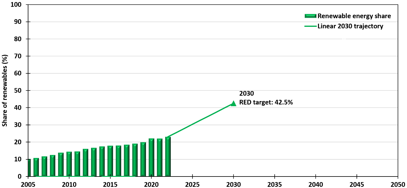
Source: Adapted from European Environment Agency (EEA, 2024b); data from Eurostat (2023b).
The building sector can contribute to this goal by promoting the integration of the production and use of renewable energy in buildings. The share of renewable energy related to the final total delivered energy demand for building operations quantifies the proportion of renewable energy used on an annual basis by a building in relation to the total delivered energy demand for the end-use energy services, i.e. heating, cooling, and dehumidification, ventilation, and humidification; hot water; and lighting (optional for residential buildings). This quantifies the percentage of the relative improvement of the share of renewable energy for the operation of a building against a baseline reference. The revised RED (Directive EU/2023/2413) sets an indicative target of at least a 49 % renewable energy share in buildings by 2030. As a result, the use of renewables for heating and cooling in buildings shall gradually increase, targeting an annual increase of the renewable energy share of at least 0.8 percentage points at national level until 2026 and 1.1 percentage points from 2026 to2030, compared to the share of renewable energy in the heating and cooling sector in 2020.
Energy storage is a crucial means to capture and store energy from renewable sources (e.g. wind, solar, or hydroelectric power) to be used later, enhancing the flexibility, stability, and reliability of an energy system, also considering the increasing share of renewable energy sources in European electricity grids. Indeed, the production of renewable energy sources is inherently variable, as it is heavily dependent from environment conditions, which fluctuate daily and seasonally. Hence, the energy storage can effectively contribute as one of the technologies that can reduce the flexibility requirements (FR) of an energy system. FR represent the energy fluctuation in relation to the average in a specific period, thereby indicating the need for technical solutions to address energy system flexibility. Three different approaches may be considered for energy storage in the EU, with specific data collected in a dedicated database of the European energy storage technologies and facilities (European Commission, 2020a), as follows:
- ‘Front of the meter facilities, including energy storage facilities in the EU, operational or in project, connected to the generation and the transmission grid.
- ‘Behind the meter’ energy storage, which refer to installed capacity per country of all energy storage systems in the residential, commercial and industrial infrastructure.
- Energy storage technologies, classified in five main categories (i.e. mechanical, electrochemical, electrical, chemical, and thermal) depending on the type of energy acting as a reservoir.
The energy storage technologies enable the storage of energy surplus during low-demand periods and provide it during high-demand periods, allowing the efficient management of supply and demand fluctuations across various timescales and facilitating grid stability. Different characteristics and capabilities offered by energy storage technologies are illustrated in Figure 7. Energy storage can be electrical, when input and output are electricity (Power-to-X-to-Power), or thermal when input and output are thermal energy, among various energy storage technologies. Electrical energy can be stored in the form of chemicals or as thermal energy (Power-to-X).
Figure 7. Discharge time vs capacity of energy storage technologies
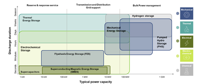
Source: EASE, 2022.
Energy storage solutions can be deployed at various spatial scales, from individual buildings to entire urban areas. At building scale, energy storage systems help to optimise the energy use, ensure a stable power supply, and are a critical enabler for increased reliance on renewables. Specifically, three typologies of energy storage systems can be considered to achieve these goals, as follows:
- Passive short-term storage, which uses the building components for thermal energy storage in the form of sensible or latent heat storage.
- Active short-term storage, which includes water tanks, ice storages, batteries (electrochemical), flywheels (mechanical), super-capacitors (electrochemical), compressed air storage (mechanical), hydrogen (chemical).
- Active seasonal storage, which refers to underground thermal energy storage or thermochemical.
At neighbourhood and urban scale, energy storage systems can enhance grid resilience, balance fluctuating energy demands, and support electric transportation infrastructure.
The increase in the share of variable renewable energy sources leads to constantly changing residual load dynamics, necessitating flexibility solutions across various timeframes. The storage solutions must align with specific timescales, ranging from short-term, like batteries offering flexibility within hours, to long-term, such as seasonal hydro storage providing flexibility over months at a city or regional scale. The flexibility requirements can be estimated based on the residual load curve, which is derived by subtracting the variable renewable supply from the power demand. The 2030 residual load curve (TWh) in the EU is expected to have two peaks, one in the morning and another in the evening, which correspond to periods of higher electricity demand. There is also a noticeable decrease during midday when solar PV generation reduces the remaining demand. The residual load curve provides insight into the portion of the electricity demand that can be covered by flexible technologies.
Figure 8. Flexibility requirements based on daily EU residual curve in 2030
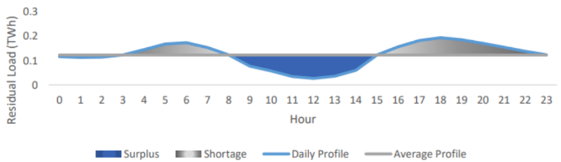
Source: Koolen et al., 2023
3.2.3 Minimise greenhouse gas emissions
The target intents to minimise whole life cycle GHG emissions that constitutes a pillar of EU policies to control the impacts of climate change. Accordingly, the target aims to achieve the two following objectives:
- Minimise the operational GHG emissions by eliminating onsite combustion of fossil fuels.
- Minimise the embodied GHG emissions for the manufacturing of building construction materials, products, components and systems.
Operational GHG emissions are mainly generated by the energy use of the building-integrated technical systems, such as space heating, domestic hot water (DHW), cooling, ventilation, and lighting during the use-phase of the life cycle of a building. The reduction of the operational GHG emissions of buildings towards zero emissions buildings is a priority to reach the EU climate-neutrality goal by 2050, in line with the GHG emission trajectory in a scenario limiting the global warming to 1.5°C above the pre-industrial levels (Figure 9), according to the Paris Agreement objectives (United Nations, 2015).
Figure 9. Trajectory for GHG emission reduction in the EU-27 in all sectors for climate‑neutrality by 2050.
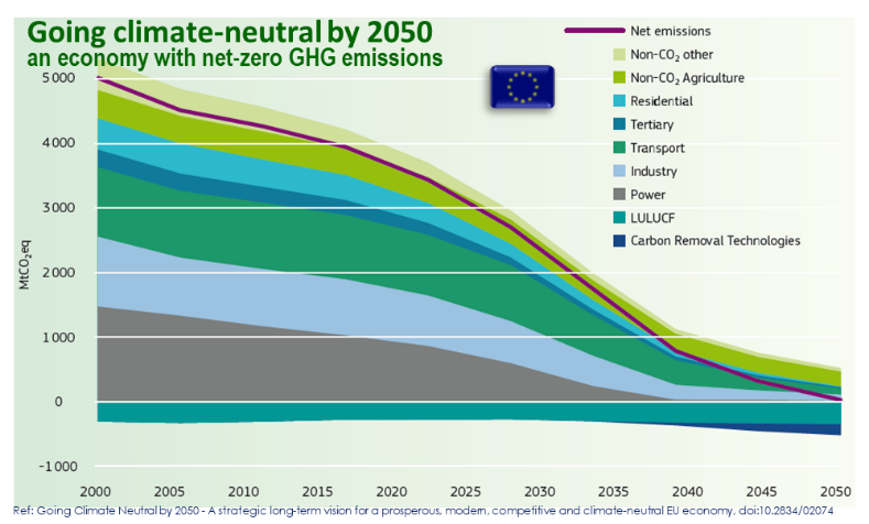
Source: European Commission, 2019.
Embodied GHG emissions of a building are generated in relation to manufacturing and processing construction products/materials used throughout the whole life cycle of a building, from “cradle” (i.e. the extraction of the raw materials for the production of construction products/materials) to “grave” (i.e. the deconstruction of the building at its end-of-life stage, along with the disposal and potential recycle/re-use of the building materials and components).
At neighbourhood and urban scale, the natural photosynthesis of urban vegetation is identified as an effective approach to capture and store carbon on site to reduce CO2 emissions, although he potential of natural photosynthesis to uptake and store carbon varies significantly depending on the plant typology (e.g. trees, bushes or herbaceous), growth conditions, climate, and maintenance methods (Kuittinen et al., 2021). In urban areas, it was estimated that the annual natural sequestration potentials from trees range from 5.9 tCO2/ha/a in Mexico to 10.3 tCO2/ha/a in USA (Shafique et al., 2020). Green roofs, which primarily reduce the energy demand of buildings helping to decrease CO2 emissions indirectly, also exploit the natural photosynthesis approach exhibiting a carbon sequestration potential that varies from 0.3 kgCO2/m2/a to 7.1 kgCO2/m2/a, depending on conditions and variables mainly related to plant types and soil layers (Shafique et al., 2020; Kuittinen et al., 2021). Nevertheless, most of this sequestered carbon is stored only for a short time, as herbaceous plants decompose naturally over growing seasons. Carbon also accumulates in soils due to organic processes, thus soils result into the largest terrestrial carbon stock. The potential of soil to store carbon varies considerably depending on climate, soil type, vegetation, erosion, microbial activity, pollution, and other factors. In urban areas, the annual amount of carbon stored in soils ranges from 213 to 741 tCO2/ha (Kuittinen et al., 2021).
3.2.4 Sustainable mobility
The promotion of the sustainable mobility is a key-aspect of the European Green Deal (COM 2019/640) to minimise the GHG emissions from transportation. Specifically, the decarbonisation of the transport sector depends on the implementation of three pillars of actions, according to the Sustainable and Smart Mobility Strategy (COM 2020/789): (i) make all transport modes more sustainable, (ii) make sustainable alternatives widely available in a multimodal transport system, and (iii) put in place the right incentives to drive the transition. These actions are essential to shift to zero-emission mobility, implying decisive measures concerning (i) the need to reduce the current dependence on fossil fuels by replacing existing fleets with low- and zero-emission vehicles, i.e. electric vehicles (EVs), also named as e-vehicles,, while boosting the use of green electricity and using low-carbon fuels, (ii) the effort to shift more activities towards more sustainable transport modes (e.g. public transportation), and other alternative active mobility modes (e.g. use of bicycles).
In this context, the building sector plays an important role in terms of necessary infrastructure for electrical recharging and cycling promotion (Directive 2024/1275), thus the assessment target aims to enhance the sustainable mobility, which can be achieved through two main efforts:
- Foster electric mobility (i.e. e-mobility), facilitating the growth of electric vehicles in urban areas by providing the necessary infrastructure for recharging EVs at both building and neighbourhood/urban scale (e.g. public recharging points for EVs).
- Encourage alternative active mobility, e.g. through the use of bicycles, by providing the necessary infrastructure at both building (e.g. bicycle parking spaces) and neighbourhood/urban scale. Regarding the neighbourhood/urban scale, infrastructure for bicycle paths and lanes should be ensured, while main emphasis is also placed on public transportation systems.
E-mobility represents another facet of the electrification era. Electric vehicles are powered by electricity from batteries. Combined with an increased share of renewable electricity production, EVs emit fewer GHG and tailpipe pollutants, compared to conventional vehicles. However, electric vehicles exhibit a limited motor and battery capacity that enables shorter-distance travels depending on the EV range. A regular and convenient access to battery recharging stations is needed to overcome this inherent drawback of EVs, thus the availability of parking facilities for recharging EVs becomes essential at both building and urban scale for an effective use of EVs. According to the EPBD recast (Directive 2024/1275), buildings shall contribute to the development of the necessary infrastructure for sustainable mobility. Specifically, the installation of recharging points, and pre-cabling or ducting need to be ensured for new and majorly renovated residential and non-residential buildings in case a car park is located inside the new/renovated building, or it is physically adjacent to the new/renovated building. The use of smart charging and bi-directional charging is recommended to enable the energy system integration of buildings. Bidirectional charging, i.e. vehicle-to-grid (V2G) or vehicle-to-home (V2H), further supports the penetration of renewable electricity by electric vehicle fleets in transport and the electricity system in general. Furthermore, the bidirectional charging is instrumental to peak shaving, thus lowering the need for power supply at peak hours and, hence, the overall system costs. Similar considerations about the need of an adequate recharging infrastructure to support e-mobility also emerge at neighbourhood and urban scale. Public and urban-wide recharging points are important not only to ensure the use of EVs, but also to provide the supply of green and low polluting electricity, contributing to both less urban pollution from GHG emissions and citizens’ wellbeing.
A shift to the alternative active mobility, such as cycling, can significantly reduce GHG emissions from transport. However, the lack of bicycle parking spaces in residential and non-residential buildings is a barrier to the uptake of cycling, also discouraging the use of bicycles (Directive 2024/1275). Hence, EU Member States shall ensure the provision of a minimum number of bicycle parking spaces for new and majorly renovated residential and non-residential buildings. Furthermore, the increase in the use of bicycles depends on the decisive factor to provide an adequate network of bicycle lanes and paths at neighbourhood and urban scale. A transportation system that is conducive to cycling can reap many benefits in terms of reduced traffic congestion and improved quality of life.
Public transportation systems are generally more energy-efficient and generate lower GHG emissions per passenger mile compared to private conventional cars. This helps mitigate climate change by reducing the overall carbon footprint of transportation. Hence, at neighbourhood and urban scale, it is essential to consider various aspects of the public transportation network concerning its extent, usage, and accessibility of the residents to boost a high-quality and multimodal transport system which takes advantage of the combination of the strengths of the different modes, such as convenience, speed, cost, reliability, predictability.
3.2.5 Non-energy related environmental impacts: air and water
The target aims to reduce the environmental impacts to air and water through two main objectives:
- Improve indoor air quality and secure the well-being of building occupants.
- Minimise water use in buildings and surface permeability in urban areas to preserve water reservoirs.
Indoor air quality can affect human health and well-being of building occupants, as it relates to sick building syndrome (SBS) and impacts indoor environmental quality, thus the need to reduce the indoor air pollution is at the EU forefront awareness. Volatile organic compounds (VOCs) emitting from construction products are an important source of indoor air pollution. However, a common regulation in the EU concerning the health-related assessment of VOC emissions from construction products still lacks, although the EU regulation on construction products (Regulation (EU) 305/2011) requires that VOC emissions must not pose any risk to the health of building users. However, the same regulation does not implement any health requirement. Accordingly, the harmonised European standards defining relevant parameters for the product performance declaration do not address VOC emissions. Hence, few EU countries, such as Germany, France, have established national requirements for VOC emissions from construction products, while the EU proceeds with the ongoing progress of a harmonised approach to communicate construction product emissions in terms of VOC classes (Scutaru and Witterseh, 2020). Outdoor air quality can impact the building indoor conditions and the quality of life in cities. The EU has also recognised the importance of this issue, thus placing emphasis on ambient air quality standards, reduction of air pollution emissions, and emissions standards for key sources of pollution. The EU zero pollution action plan (COM 2021/400) sets the ‘2030 Target’ to reduce the health impacts of air pollution (the number of premature deaths) by more than 55 % compared to the 2005 levels and the ‘2050 vision’ to reduce air, water and soil pollution to levels no longer considered harmful to health. European standards include reference methods for sampling and measuring the following indoor pollutants: PM10 and PM2.5 in ambient air according to EN 12341 (CEN, 2023), ozone according to EN 14625 (CEN, 2012a), sulphur dioxide according to EN 14212 (CEN, 2012b), and nitrogen dioxide according to EN 14211 (CEN, 2012c). Moreover, the Air Control Toolbox provides practical European air quality forecasts (Copernicus n.d.) like the air quality models that are also available from the Support Center for Regulatory Atmospheric Modeling in the United States (EPA n.d.). Accordingly, it is important to minimise the potential intake of outdoor particulate and gaseous pollutants to the ventilation system. Potential solutions to minimise the intake of outdoor air pollutants (e.g. fine dust and benzene) could be to place the ground level air intakes on the side of the building that is exposed to the carpark, thus avoiding the building sides exposed to the main road, and to provide the sheltering of ground-level air intakes by a row of densely planted trees. The indoor generation of air pollutants (e.g. off-gassing of VOCs from fit out materials or insulation) can be minimised by selecting and using low-emission materials. Each individual VOC has its own potential toxicity upon exposure to humans. The building ventilation strategy with clean outdoor air can also play an important role to freshen up the indoor air, thus reducing indoor air pollution. A hybrid ventilation system can be effective where natural ventilation provides sufficient air change rates for emissions from building components and occupants during low occupancy periods, while mechanical ventilation can be used during periods of normal and high occupancy. The mechanical ventilation system should be able to provide a safety margin against the build-up of VOCs from fit-out materials/furnishings and against the remaining of bio-effluents in indoor air. Localised ventilation strategies can be used to control point sources in areas of the building (e.g. cooking areas, bathrooms, meeting rooms with occasionally high occupancy) and consider a separate exhaust, for defined time periods, with a high specific ventilation rate.
Water availability is unevenly distributed in Europe, despite the relevant abundance of freshwater resources, thus leading to major differences in terms of water stress for the European population over seasons and regions. Although the overall use of water resources can be considered sustainable in the long-term in most of Europe, specific regions, particularly in southern Europe, may face serious challenges related to water scarcity and seasonal water shortages. Hence, a more efficient use of water will also reduce pressure on freshwater resources, especially in river basins that experience continual or seasonal water scarcity. In areas where the desalination is necessary for water supply (especially in southern Europe), the cost and environmental impacts for an efficient water use are significantly higher due to the larger amount of energy needed to treat the water. An average of 144 litres of freshwater per person per day is supplied for the European household consumption, which is almost three times the water requirements for basic human needs (EEA, 2018). Reducing water consumption at building scale will lessen the environmental impacts of delivering water to the point of demand (i.e. from water abstraction, treatment and pumping through the distribution network), thus sustaining a healthy natural environment, while meeting human needs (Directive 2000/60/EC). In the case of domestic hot water, better efficiency also leads to significant energy savings for consumers. The trend towards larger urban populations is placing even more pressure on water supply at urban scale. Furthermore, surface permeability should be ensured in urban areas, as it is an important environmental characteristic for the natural water cycle. However, the extent of impermeable surfaces in urban areas is continually increasing, as cities expand due to the construction of buildings, roads, streets, parking lots, etc. to rapidly adjust to population growth. As a result, surface imperviousness increases with the consequent increase of the volume and velocity of surface runoff and the reduction of water infiltration, which can also lead to floodings. In this context, the EU soil strategy for 2030 (COM 2021/699) provides a framework and relevant guidelines to mitigate, limit or restore the sealed soil areas.
3.2.6 Non-energy related environmental impacts: construction materials
The EU is committed to circular economy, emphasising resource efficiency and waste reduction to minimise the use of raw materials, energy, water, also lessening GHG emissions. In this context, the target addresses environmental impacts related to construction materials through the following objective:
- Minimise waste from building construction and demolition activities.
The construction and demolition waste (CDW) management in the EU is closely intertwined with the overarching goal of the decarbonisation strategy. Over 2 tonnes of CDW are generated for each European citizen on an annual basis, accumulating about 500 million and 1 billion tonnes (EU Construction n.d.). As a result, CDW accounts for more than a third (i.e. 35 %) of all waste generated in the EU (COM 2020a/98). Based on these figures, it is not surprising that CDW is a priority waste stream under the Waste Framework Directive (Directive, 2008/98/EC) aiming to increase the preparing for re-use, recycling and recovery of non-hazardous CDW to a minimum of 70 % (by weight) by 2020, promote selective demolition, establish sorting systems and reduce waste generation. In this context, sustainable construction practices that prioritise the reduction of CDW through recycling and reuse should be applied to both the new construction and the renovation of buildings. In fact, renovation works also generate CDW since the intervention may also involve the structural alteration of buildings, replacement of main services or finishes, while at the same time including associated redecoration or restoration works.
3.2.7 The role of the economic involvement of public sector
The public sector investments in buildings or living spaces often aim to transform places or enhance the functions provided to the community, thus supporting the economic development, stimulating economic growth, creating jobs, and attracting more investment to the transformation project area. In this context, the assessment of the use and performance of potential public investments become particularly relevant for a project in line with the NEB vision.
Traditionally, evaluation frameworks, such as cost-benefit analysis (CBA) and cost-effectiveness analysis (CEA), have been used to assess the viability of a public investment. However, in recent times, the social return on investment (SROI) methodology has been promoted as a more holistic approach to demonstrating the social, economic, and environmental values, expressed in monetary terms, to provide a comprehensive view of the benefits to people and nature created by the investment cost. Furthermore, economic activities aligned with environmental policies have been encouraged through the introduction of the ‘Do No Significant Harm’ (DNSH)-principle, which aims to avoid investments or reforms that would cause significant harm to the six environmental objectives defined in the EU Sustainable Investment Regulation (Regulation 2020/852), thus achieving environmentally-sensitive management of public finance.
The Cost-Benefits Analysis (CBA) is an analytical tool that assesses the variation in social welfare resulting from an investment decision (usually related to land or infrastructure development) and, consequently, its contribution to achieving the objectives of a project or an overarching policy. A CBA relies on the assumption of allocating resources for a project until the marginal social benefit equals the marginal social cost. Hence, a project or a policy can be considered valid from a societal point of view, if the benefits generated exceed the costs. A CBA aims to facilitate a more efficient allocation of resources by demonstrating the convenience of a particular intervention for society compared to other possible ones. The CBA evaluates the purely financial convenience of a project, assesses the necessary financial backing, and identifies any participation in the backing by the users. The financial performance evaluated through a CBA relies on the following project investment criteria, which measure the profitability of a project:
- The net present value (NPV) is given by the difference between discounted benefits (B) and costs (C) at a given discount rate (r), over the project lifetime (T) in years, according to Equation (4):
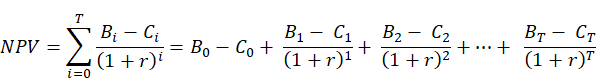
(4)
If the NPV is positive, the social benefits are higher than the social costs. If the alternative is the status quo with zero costs and benefits, a positive NPV indicates that the project can be implemented. By comparing different options for a project, having the same investmentsize, the solution with a higher NPV is preferred.
- The internal rate of return (IRR) is the discount rate that would make the current value of a project equal to zero (NPV = 0), namely the discount rate that allows the value of the initial investment to be recovered at the time (T). Based on this, a project is eligible, if it exceeds the opportunity cost of the investment. The reference is usually taken as a non-risky investment (e.g. bank deposit). By comparing different projects, the option with a higher IRR is preferred.
- The cost-benefit ratio (B/C) is given by the ratio between the sum of the benefits and the sum of the costs. The ratio must be greater than one (i.e. B/C > 1) to consider a project eligible. The ratio between the sum of the benefits and the sum of the costs must preferably be carried out by considering discounted values.
- The discounted payback period (DPBP) is a more accurate version of thesimple payback period. The latter measuresthe amount of time (expressed in years) required to fully recover the initial cost of a project from the net annual cash inflows coming from the profits of the project implementation, without accounting for the time value of money. Indeed, the calculation of the simple payback period does not include the discount rate, whereas the DPBP takes into account the cumulative annual discounted cash inflows to equal the amount of the initial investment.The shorter the payback period, the more cost-effective the project is. However, either the simple or the discounted payback period is more relevant in the private sector than in the public sector.
It is possible that a project delivers a positive economic return in terms of social well-being, but this result is a loss from a purely financial point of view due to fragmented financial indicators that do not represent the overall economic value of the project. However, the social benefits generated can make the project worthwhile. As example, the realisation of a green area in a district has certainly a negative economic return since the costs of construction and management are not covered by any monetary revenue from users. However, the social benefits to the local community are relevant. In that case, integrative assessment frameworks, such as SROI, should be considered.
The Cost-Effectiveness Analysis (CEA) is a tool for evaluating public projects or policies, particularly applied in the sectors of health, road safety, national defence, or energy efficiency. CEA identifies the most efficient way in economic terms to achieve a given objective. It is generally preferred to a CBA by non-economically trained analysts (e.g. engineers, doctors, etc.), who may be less inclined to accept the controversy of monetising the benefits of "intangible" goods, such as human life, time, health, or environmental services, which a CBA requires. The CEA is also applied by economists who did not recognise the underlying social welfare approach of a CBA. In the CEA only the direct costs invested in the project are considered. At the same time, the effectiveness is measured through a single outcome, which stands as the main expected impact of the intervention and is used to compare costs and the impact of alternatives within the same domain. It does not evaluate the monetary value of the outcomes asthey are reported as natural units (e.g. lives saved, or cases averted). Similarly to the CBA, stakeholders are not involved in the process; the evaluator defines the main objective of the intervention and its impact. A CEA can be applied as an ex-ante evaluation to steer the decision-making process or as an ex-post evaluation of an intervention. When selecting alternatives, the intervention with a higher cost-effectiveness ratio is better. If the project outcome cannot be defined as a priority outcome or if homogeneous and quantifiable units cannot be determined, cost-effectiveness analysis should be avoided. The typical criterium of a CEA is the incremental cost-effectiveness ratio, defined as the ratio of change in costs to the change in impacts. A classic and interesting example of a cost-effectiveness analysis is the marginal abatement cost curves, used to visualise the abatement cost and the abatement potential of CO2 emissions.
The social return on investment methodology is a framework for measuring and accounting for a much broader concept of value created by a project/activity (Nicholls et al., 2012). SROI seeks to prevent inequality and environmental degradation, and improve well-being by incorporating social, environmental, and economic costs and benefits to indicate how the change due to a project/activity is being created. SROI was initially developed and used to evaluate social investments, such as programs for combating drug or alcohol abuse, supporting job search, and reducing the need for social assistance and empowerment. Recently, it has also begun to be used in evaluating complex urban programs, where activities in the built environment interpenetrate with those related to service delivery (Watson and Whitley, 2017). A SROI analysis may be carried out in two different forms: (i) as a ‘SROI forecast’, thus being an ex-ante evaluation which predicts the extent of the social value of a change that will be created if the project/program meets its intended outcomes, and/or (ii) as an ‘evaluative SROI’, which is an ex-post evaluation performed retrospectively and based on actual outcomes that have already taken place. Although the SROI methodology can be categorised as a form of cost-benefit analysis, a crucial distinction between a CBA and an SROI analysis regards the evaluation object. Specifically, a CBA takes as main evaluation object the outputs of the intervention (e.g. the physical, digital or natural infrastructure provided to a city against its cost). At the same time, a SROI analysis focuses on welfare changes experienced by stakeholders in being involved in a project/program and benefitting from its result (e.g. the outcomes that the existence of the physical, digital or natural infrastructure or the participation to its implementation during the co-design process delivers to a specific group of people, regardless its role in the process). Outputs are obvious in CBA and SROI, while outcomes in SROI should be defined by the analyst interacting with stakeholders. The general performance indicator of SROI is the ratio of the social return gained (B) translated into a monetary value to the initial investment (C), i.e. B/C. Methods and techniques for translating impacts into monetary values may be similar to the ones used in a CBA for non-market values. A further crucial practical consideration is the staff time and effort required to undertake a CBA or SROI analysis. Implementing an SROI analysis is relatively feasible when an organisation collects information on program outcomes, cost, and revenue.
The suitability of the evaluation frameworks and tools above to assess public investments for buildings, living spaces, infrastructures, and services is summarised in Table 2.
Table 2: Evaluation frameworks and tools for public investments.
| Evaluation tools | ||||
| Buildings | Living Spaces | Infrastructures | Building services | |
| CBA | √1 | √1 | ||
| CEA | √1 | √1 | √1 | |
| SROI | √2 | √1 | √3 | √1 |
| DNSH | √4 | √4 | √4 | |
1 Suitable for evaluation.
2 It is suitable for evaluation when there is a combination of tangible (i.e.'hard investment', such as infrastructure, construction, etc.) and intangible goods or services (i.e. 'soft investment', such as human life, time, health or environmental services, etc.) for people.
3 Suitable for evaluation but not frequently used.
4 Suitable for evaluation only for 'hard investment', mandatory for interventions financed by National Recovery and Resilience Plans.
Source: JRC.
Beyond the public investments for which future benefits are inherently expected, public fundings may also reveal particularly relevant for projects in line with the NEB vison, mainly to support local transformations. In this context, the performance of fundings also needs to be evaluated and the funding accountability should be enhanced, so it is crucial to clearly present funding mechanisms and their figures in the design phase of a project. This includes detailing the financial resources to support a project and their contribution to the economic development. By outlining funding sources and amounts, stakeholders can better understand the impact of an investment on local economies.
3.2.8 The role of the economic involvement of the private and finance sector
A key-aspect to support NEB projects relies on the development of specialised financial products and investments from the private sector. Traditional financial instruments may not adequately address the unique characteristics of projects aligned with the NEB vision, which generally blends aspects of sustainable technologies, functionality and aesthetics, and community engagement. This drawback can be overcome by considering new financial instruments in the form of debt (i.e. bonds and loans) or equity (i.e. funds) for sustainable growth-oriented projects, such as green loans, sustainability bonds, and impact investment funds, to be specifically designed for projects compliant with the NEB vision. These financial products would ensure the flow of capital towards these initiatives and reinforce the growing importance of sustainable finance, which is generally referred to as the process of integrating ESG criteria into investment decisions within the private sector (Boffo and Patalano, 2020). Particular attention within sustainable finance is drawn up to the environmental subset of sustainable development in line with the European Green Deal objectives, leading to the environmental (or green) finance that concerns private financing only focused on ecological issues aimed at optimising environmental benefits or reducing and/or adapting to environmental risks, as a complement to public investment. Specifically, green finance supports the transition to a climate-resilient economy through (i) carbon finance enabling climate-change mitigation actions, especially related to the GHG emissions reduction, and (ii) climate finance for climate-change adaptation efforts towards promoting the climate resilience of infrastructure. Applications of carbon finance include low carbon projects, such as projects for the reduction of GHG emissions from deforestation and forest degradation (REDD+), whereas applications of climate finance regard clean energy and energy efficiency projects, as well as climate change adaptation projects, such as building flood defences to warming waters. In private climate finance, various financial tools are utilised, including environmental, social, and governance funds with a focus on climate considerations, private equity investments, and venture capital injections into climate-related businesses. Additionally, shareholder engagement is employed to encourage companies to make environmentally responsible investment decisions. Beyond climate-related issues, green finance also channels capital into projects addressing other environmental issues (e.g. related to air, soil, water, etc.). The involvement of private sector capital in climate finance should be enhanced, with a particular focus on innovative financial tools. An increasing number of institutional investors, investment funds, and credit institutions have begun to address climate change and sustainability. Various financial instruments have seen an increasing use in climate finance in recent years. This trend has incentivised financial institutions from the private sector to explore climate‑related offerings and collaborate with public-sector entities and multilateral development banks (MDBs) to create joint initiatives and partnerships. Major global investment funds can initiate investments in climate financial products within emerging markets and developing economies (EMDEs) by allocating a portion of their capital and diversifying their risk. These funds can collaborate with MDBs and national public sector organisations by dedicating a portion of their portfolio to climate-focused EMDE products and projects, aligning with their climate commitments and the preferences of their investors. An overview of the predominat new financial instruments within the various facets of sustainable finance, along with their main application to relevant projects, are reported by finance category in Table 3.
Table 3. Financial instruments within sustainable finance
| Financing tool | Definition | Application | References |
| Climate and green finance | |||
| Climate bonds | Fixed-income financial instruments that are linked with climate change solutions. They are issued to raise finance for climate change solutions for mitigation- or adaptation-related projects | Climate change mitigation projects mainly related to GHG emissions reduction, such as clean energy and energy efficiency projects. Climate change adaptation projects, such as building flood defences to warming waters. | Lucchetta (2023) |
| Green bonds | Any type of bond instrument where the proceeds are exclusively applied to the finance or re finance of projects with clear environmental benefits (some projects may also be eligible for a ‘green’ designation) | Green projects, such as renewable energy, energy efficiency, pollution prevention and control, terrestrial and aquatic biodiversity conservation, clean transportation, sustainable water and astewater management, climate change adaptation, eco-efficient and/or circular economy, and green building projects. | Bhutta (2022) |
Green loans | Any type of loan instrument made available exclusively to finance or re finance, in whole or in part, new and/or existing eligible green projects | Same applications as indicated for ‘green bonds’. | Mirovic (2023) |
| Green funds | Funds (equityfinancing) that provide clients with platforms through which environmentally friendly businesses and organisations are supported with long term funding | Climate change and environmentally friendly projects, such as energy efficiency, agriculture and waste management projects. | Silva (2016) |
| Green credits | Green deposit, mortgage, and project loan from lending industry
| Environmental protection, emission reduction, and energy conservation projects; green industries. Investment restriction to high-pollution, high-emission and overcapacity industries, and withdrawal of financing from prohibited industries primarily targeted for their negative environmental impact. | Esposito (2022) |
| Green banking | Green banking facilitates private investments in domestic low-carbon, climate-resilient infrastructure and other green sectors, such as water and waste management. | Meeting ambitious emissions targets, creating jobs, supporting local community development, mobilizing private capital, energy efficient street | Sharma (2022) |
| Green asset-backed securities (ABSs) | Green securitisation involves the conversion of illiquid climate- or green-friendly assets into tradable financial instruments (i.e. securities). | Low-carbon projects | Lei (2024) |
| Social finance | |||
| Social Impact Bonds | Investment contract with the public sector to achieve financial return on investment, while meeting desired social outcomes. | SROI projects, including community investing, affordable infrastructure (e.g. alternative/clean energy technologies), affordable housing and loans, human rights, political and social activism, and religious value | Solntsev (2021) |
| Sustainable finance | |||
| Sustainability (socio-environmental) bonds | Any type of bond instrument where the proceeds or an equivalent amount will be exclusively applied to finance or re-finance a combination of both green and social projects | SROI projects, including community investing, affordable infrastructure (e.g. alternative/clean energy technologies), affordable housing and loans, human rights, political and social activism, and religious value | Mocanu (2021) |
Sustainability-linked bonds and sustainability-linked loans | Any type of bond and loan instrument employed by companies and governments to secure capital, often at reduced costs, by committing to achieving predefined sustainability/ESG objectives. | SROI projects, including community investing, affordable infrastructure (e.g. alternative/clean energy technologies), affordable housing and loans, human rights, political and social activism, and religious value | Mocanu (2021) |
Source: JRC.
Tailoring the aforementioned new financial products for the NEB also involves rethinking risk assessment models. Traditional models may not accurately capture the complexity of NEB projects and potential long-term benefits. Financial institutions must develop new frameworks for evaluating risks and returns that consider environmental impact, social value, and long-term sustainability. Moreover, offering insurance products and guarantees can help mitigate the perceived risks associated with innovative and sustainable projects. Another crucial aspect is the establishment of investment funds dedicated to supporting NEB projects. These funds would pool capital from investors interested in contributing to sustainable and socially impactful projects, providing a steady financing stream. Furthermore, these funds could offer technical assistance and expertise to projects, ensuring their success and alignment with the NEB vision. Financial tools and models influencing the private and finance sector to effectively support NEB projects are described, as follows:
- Public-private partnerships (PPPs) can play a significant role in financing NEB projects. These partnerships (e.g. social impact bond) could leverage public funds to attract private investments, thus reducing the financial burden on both parties, while achieving public interest goals. PPPs can be particularly effective in large-scale urban development projects that embody NEB principles. Although PPPs offer numerous advantages, challenges, such as aligning divergent goals, ensuring transparency, and managing public expectations, need to be considered. Overcoming these challenges requires clear communication, shared objectives, and strong governance structures. Trust is a fundamental component of successful PPPs, necessitating consistent and open dialogue between public and private partners and with the communities they serve.
- Community-based financing models, such as crowdfunding or community bonds, can mobilise resources for local projects aligned with the NEB values. These models not only provide the necessary funding, but also foster a sense of ownership and engagement among community members, aligning perfectly with the NEB emphasis on inclusiveness and community involvement.
- Government incentives can be a powerful tool in encouraging investments in NEB projects. Tax breaks, subsidies, or grant programs for sustainable and inclusive building projects can make them more financially viable and attractive to investors. Governments can also provide seed funding or matching funds for NEB-aligned projects, drawing particular attention on experimental or community-oriented projects.
However, in the EU evolving financial framework, small and medium size enterprises (SMEs) and even smaller businesses, which are vital for the EU economy and crucial for strategic investments, resilience, and decarbonisation, still rely on bank financing for their operations and innovation. Banks facing economic uncertainty and rising interest rates require a long-term financial instrument for stable funding and efficient asset liability management. Furthermore, in the last years theincreasing requirements for EU taxonomy and ESG factors disclosure for large companies and listed SMEs that are required by the Corporate Sustainability Reporting Directive (CSRD) (Directive, 2022/2464) to regularly report on the social and environmental risks they face, and on the impact of their activities on people and environment, according to the European Sustainability Reporting Standards (ESRS) (Commission Delegated Regulation, 2023), create further challenges for obtaining investments, as investors can access company data more easily, potentially influencing their investment decisions. ESG data is even more critical for micro-enterprises, and various public and private initiatives aim to collect and score ESG data for small businesses. An example in this direction refers to the Energy Efficient Mortgage Initiative (EEMI) which aims at implementing the ESG best practices in the financial sector in support to the objectives of the EU Green Deal and Renovation Wave strategy by channeling the private finance towards investment in energy efficient buildings and energy saving renovations. The EEMI has introduced a specific ‘harmonized disclosure template’, enhancing the overall ESG disclosure for cover pools. ESG has gained prominence in capital markets, but its adoption in covered bond markets has been relatively limited due to data constraints on the ESG attributes of balance sheet assets. Banks have often chosen to use ESG-compliant loans for other types of issuance, like senior preferred or tier 2 bonds, rather than covered bonds. The diversity of investment approaches for applying ESG factors is evident, with only around half of all investment approaches having a specific ESG mandate covering covered bonds. Some investors rely on the issuer's designation of green or social bonds, while others consider issuer’s sustainability ratings, a combination of both, or rely on internal models. In recent years, ESG criteria have become increasingly integrated into issuer and covered bond rating methodologies. This integration is based on how ESG factors impact issuer or bond credit risk. Additionally, external reviewers assign ESG ratings or scores to banks based solely on their ESG performance. Issuers can also obtain external assessments of their green, social, or sustainability bond processes, including four types of bond-related reviews identified by the International Capital Market Association (Karoui, 2024), as follows:
- Second-party opinion (SPO): Independent institutions assess the quality of a sustainable bond framework and verify its alignment with relevant principles. For example, Institutional Shareholder Services (ISS ESG) and Sustainalytics often provide second-party opinions for sustainable covered bond frameworks.
- Verification: post-issuance, external auditors often verify the allocation of proceeds, sometimes in conjunction with SPO providers.
- Certification: issuers can obtain certification of their green, social, or sustainability bonds against recognised external standards or labels. For instance, some green covered bonds are certified by the Climate Bond Initiative to ensure alignment with the goals of the Paris Agreement.
- Green, social, and sustainability bonds, and sustainability-linked bond scoring/rating, which assess the performance of issuers or bonds in terms of ESG factors. Imug and ISS ESG are examples of rating agencies that provide such ratings.
In the primary market, ESG-labelled covered bonds tend to attract larger order books and higher cover ratios than conventional counterparts. However, data on new issue premiums are inconclusive. In 2022, ESG-labelled covered bonds had an average new-issue premium 0.4 basis points lower, while in early 2023, it was higher by the same margin. Thus, the pricing advantage associated with an ESG label appears minimal or non-existent for covered bond issuers. Nevertheless, larger order books reduce execution risk and could contribute to more stable secondary-market performance, as ESG investors are often seen as more loyal
Social and sustainability covered bonds maintain the same high security standards and risk profiles as regular covered bonds, resulting in no significant price difference between comparable issues. However, there could be minimal variations influenced by the broader investor base and increased demand for social and sustainability covered bonds. Determining the relative value of social and sustainability covered bonds compared to regular covered bonds is challenging due to several factors. Covered bond spreads, in general, are compressed, offering limited room for differentiation. Moreover, many issuers do not have bonds with matching tenors in both social/sustainability and regular categories
3.2.9 Circular Economy
Natural resources scarcity is a key‑factor that affects the effectiveness and continuity of economy and production. Overproduction in modern economies to meet the growing needs and desires of the rapidly increasing population requires huge amounts of natural resources which are in gradual depletion. In these conditions, many attempts and initiatives have been undertaken to reduce or even eliminate the consumption of natural resources, to slow the use of materials and to close the cycles of waste materials. These attempts are lately placed under the concept of circular economy that implies that any actor of an economic system should adjust its behavior from a linear to a circular thinking. Engineering principles could assist in closing or slowing the loop of materials such as cradle-to-cradle, performance economy, and industrial ecology.Currently, CE concept has gained great recognition as an effective tool, method, technique, and theory to achieve win–win solutions, such as economic opportunities and environmental protection.The main goal of CE is to shift the focus of the current production system from the linear logic of “take, produce, consume and dispose” to “close the loop”, where the end-of-life products return to the production stage and interventions are made throughout the technical or biological cycles of materials.
The existing broad and well-established link between the built environment and the economic development has caused a tremendous impact on the natural environment and the ecosystems. Specifically, the current development model of the use of resourcses within the built environment is largely unsustainable for three main reasons: (i) the depletion of finite natural resources, whereas almost 90 % of all materials extracted and used are wasted, (ii) GHG emissions that accelerate climate change, and (iii) the inequities and human rights challenges (WGBC, 2023).The construction industry is also a major economic activity in Europe while it consumes about 1094 million tons of materials, withthe residential sector consuming almost three times the amount of the non-residentialsector (CBC, 2023). The EU generates 124000 kilotons of demolition waste. Of all the construction materials that are processed as waste, roughly 71 % are recycled or backfilled, while about 10 % of construction waste is landfilled and 0.2 % is incinerated (Eliote and Leite, 2022; Munaro et al., 2020). The construction industry is also exposed to high prices, extended linear supply chain disruptions and global volatility. Although construction materials represent one of the main inputs in the construction process, recent prices of input materials have very closely correlated with construction output prices in the EU (Figure 10).
Figure 10. EU construction prices and costs during the period 2005-2023
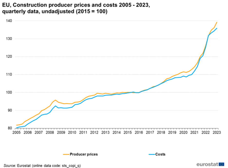
Source: Eurostat (sts_copi_q)).
Based on these figures, the transition to a circular economy within the built environment is urgent to ensure resource efficiency and also provide opportunities to decouple economic growth from carbon emissions. Increasing the EU circular material use rate (CMUR) can reduce the use of natural resources and extracted materials and minimise the negative environmental impacts. A progressive increase in the amount of use of materials coming from the waste recycled has slightly raised the EU-27 average from 10.7 % in 2010 to 11.5 % in 2022 (Eurostat, 2023c). However, the 2022 rate is still considered low as the EU target to double the CMUR by 2030, compared to 2020 rate, corresponds to a CMUR equal to 23.4 % by 2030. In this context, a circular building is defined as a building that “optimises the use of resources whilst minimising waste throughout its whole lifecycle” (WBCSD, 2021), thus circular buildings should be designed to reduce waste and pollution, while promoting the reuse of construction products and materials, and facilitating the regeneration of natural systems, according to three main CE principles, i.e. (i) eliminate waste and pollution, (ii) circulate products and materials, and (iii) regenerate nature (Ellen MacArthur Foundation, 2021). However, the measurement of the circularity level of a building still remains a complex issue. The implementation of the aforementioned three CE principles to the built environment may address this challenge by identifying specific measurements needed to align to each principle and determining relevant actions to improve circularity (WBCSD, 2022a), as summarised in Table 4. Further analyses and findings concerning the circular economy within the built environment can be found in relevant reports indicated in Annex A.
Table 4. Circular principles applied to the built environment.
| Circular principle1 | Measurements and actions |
1. Eliminate waste and pollution
| Measure emissions, and air, land and water pollution, as well as structural sources of pollution, such as traffic, to be considered for the in-use stage of a building, but also for different life cycle stages, such as construction, maintenance and demolition. |
2. Circulate products and materials.
| Measure and reduce energy, labor and material use across a building lifecycle, thus considering how the building is being used and how this use could be extended and dematerialised. |
| 3. Regenerate nature. | Measure the use of renewable materials and energy, with particularattention upon the materials regenerative in nature. |
1 CE principles as defined in Ellen MacArthur Foundation (2021).
Source: Adapted from WBCSD, 2022a
Other barriers to be faced when designing a circular building mainly concern the adoption of materials with circular features due to cost competitiveness, complex certification processes and lack of appropriate regulations that do not incentivise the use of alternative materials compared to traditional ones (WGBC, 2023). The current lack of standardisation also results in the need for various certifications, which are costly and time-consuming. Currently, there is no uniform circularity standard for a project evaluation and assessment, which further complicates the identification of the ‘value’ of a circular building for an investment portfolio, thus resulting into a higher risk and less transparent sector than the traditional building sector (CBC, 2023). However, in 2021 a standardisation effort was initiated at European level, by establishing the subcommittee (SC) of the Technical Committee (TC) 350 of the Comité Européen de Normalisation (CEN), i.e CEN/TC 350/ SC 1 – Circular economy in the construction sector, to develop standards in the field of circular economy in the built environment aimed at providing principles, guidelines, and requirements to facilitate the transition to a more sustainable circular economy in all stages of life cycle of construction projects. This ongoing work will consider the standardisation effort carried out at international level by the TC 323 of the International Organization for Standardization (ISO), i.e. ISO/TC 323 - Circular economy, to develop six new standards to foster the shift towards a circular economy by developing frameworks, guidance and requirements for the implementation of circular economy activities of organisations. Specifically, four out of the six standards are currently published, focusing on (i) the definition of key terms, concepts and guidance applicable to any type of public or private organisation, i.e. ISO 59004 (ISO, 2024a), (ii) business-oriented strategies to implement circular economy practices at both organizational and inter-organizational levels, i.e. ISO 59010 (ISO, 2024b), (iii) a framework, applicable at regional, organizational, inter-organizational or product level, to measure and assess the circularity performance based on mandatory and optional indicators, i.e. ISO 59020 (ISO, 2024c), and (iv) the review of characteristics of value networks as examples in accelerating the circular economy transition, i.e. ISO 59032 (ISO, 2024d).
Additionally, another barrier towards a consolidated approach to the circular design of buildings concerns the lack of examples and case studies integrating more than one aspect of the circular economy. Currently, it still seems complex to find project analyses in which different resources (e.g. materials, energy, and water) are considered and monitored at the same time in a circular approach. Even when very few demonstration projects in this direction are available, they are usually developed at a small scale, which is ineffective in drawing any robust conclusion on circularity performance assessment. Hence, investment in circular building projects at least at neighbourhood or larger scale are needed to demonstrate and measure the circularity benefits. However, recently interesting steps to overcome this gap at building scale have been carried through case studies available for Level(s) in its eLearning modules[1] explaining the principles and concepts for applying circular economy principles in our built environment. Another example in this direction is the 2019-2022 Life for LCA LCC Level(s) project[2] (also known as LIFE project) directed towards mainstreaming sustainable buildings in Europe through greater awareness and use of the specified indicators, i.e. Life cycle assessment (LCA), Life cycle costing (LCC) and Indoor air quality (IAQ), within the framework of Level(s). The idea behind the LIFE project is to work with stakeholders form the public, private and certification schemes to explore how the mentioned key Level(s) indicators can be implemented on a pan-European scale for building assessment.
[1] Level(s) eLearning: https://academy.europa.eu/courses/level-s-sustainable-performance-in-buildings
[2] LIFE Level(s) project: https://lifelevels.eu/
3.3 Selection criteria and list of KPIs
A detailed literature review was first carried out to identify and map relevant scientific areas and criteria addressing environmental issues related to the built environment in line with (i) relevant Sustainable Development Goals (SDGs) of the United Nations (UN) 2030 Agenda for Sustainable Development (UN, Resolution 2015), including the SDG 6 to preserve clean water, the SDG 7 for affordable and clean energy, the SDG 11 for sustainable cities and communities, and the SDG 12 for responsible consumption and production patterns through resource and energy efficiency, and (ii) EU efforts contributing to the implementation of these goals through policies and initiatives (Eurostat, 2024) channelling global environmental challenges.
The selected KPIs and their corresponding indicators relevant to the environmental perspective of the Sustainability dimension were derived from a plethora of indicators and metrics that are commonly used in voluntary and commercial rating systems, also known as green building rating systems, based on a multi-criteria approach providing the sustainability assessment of a building to award a corresponding certificate (Mattoni et al., 2018). Specifically, the investigation was focused on both European, e.g. BREEAM[1] (UK), ITACA Protocol[2] (Italy), and non-European, e.g. LEED[3] (USA), Green star[4] (Australia), CASBEE[5] (Japan) rating systems, along with standards on green building design, such as the ASHRAE Standard 189.1 (ASHRAE, 2023a). The work also aligned with Level(s), which is a voluntary reporting framework developed by the European Commission in 2020 to improve the sustainability of buildings based on a common system of indicators (Dodd et al., 2021a). Level(s) is being used in EU policy and other instruments like the EPBD, taxonomy and green public procurement, while impacting commercial certification schemes (Donatello et al., 2022).
Indeed, the heterogeneity of the available rating systems leads to various drawbacks, such as the difficult comparability of the final score of an assessment. Moreover, the rating systems include distinctive local features specific of the regional characteristics of the area where the tool was developed, limiting their application globally. Only few rating systems provide international versions enabling their application by other countries or regions apart from the origin country, such as BREEAM, and LEED, thus Level(s) represented a significant attempt to overcome the difficulty of managing the extensive heterogeneity of the existing certification schemes. Level(s) effort to develop a holistic transparent and regionally adaptable tool supports circular economy principles in the built environment across the whole life cycle of a building, focusing on GHG emissions, resource efficiency, and water use. Level(s) complements the NEB initiative by identifying measures to improve the sustainability of European buildings at each stage of their life cycle.
The selection criteria for the economic aspects of the Sustainability dimension of the NEB paradigm mainly concerned a review of relevant frameworks and tools for greening the public sector focusing on the promotion of public investments in low emission assets and green economy, as well as on the implementation of decarbonisation activities. Other analyses referred to the social return of investment methodology and the economic spillover effects of the public investment. Indicators incorporating green financial tools, the financing of sustainable real estate investments, as well as the promotion and implementation of ESG factors and investments were analysed with reference to the greening of private and finance sector. Finally, studies on the degree of circularity of materials were investigated to elaborate relevant indicators fostering the circular economy within the built environment.
Following the review and analysis phase, the final selection and elaboration of relevant indicators, reflecting the sustainability priorities within the NEB initiative, came as a result of various efforts to (i) converge to a manageable number of commonly used indicators, (ii) identify consistently measurable indicators based on relevant standards, well established common practices and other consolidated methodologies, and (iii) ensure the development of quantitative indicators. As a result of this process, nine KPIs have been developed within the Sustainability dimension to evaluate the specific assessment targets at the different spatial scales, types, and main uses of a project.
The KPIs within the Sustainability dimension together with the associated indicators and indicator weights (wS.i.j) are provided in Table 5 that also reports the KPI weights (wS.i). The same table also presents the field of application and consideration of indicators according to the project classification based on scale, type, main use and relevance to cultural heritage.
Additional information on each KPI is provided in Sections 3.4-3.12, including the rationale, background, calculation method, and input data needed for the evaluation. The calculation method addresses the evaluation of indicator scores, KPI scores and KPI performance classes according to Sections 2.2.1 and 2.2.2.
Table 5. Key performance indicators (KPIs) within Sustainability.
| KPI1 | Weight (wS.i.) | Indicator | Scale | Type | Main use | Cultural heritage2 | Weight (wS.i.j) |
|---|---|---|---|---|---|---|---|
Minimise
| 0.15 | Primary energy demand (S.1.1) | Building | Newbuild | Residential | Not affected | 0.3 |
| Electricity peak demand (S.1.2) | Not affected | 0.45 | |||||
| Smart readiness for buildings (S.1.3) | Not affected | 0.25 | |||||
| (S.1.1) | Building | Newbuild | Non-residential | Not affected | 0.25 | ||
| (S.1.2) | Not affected | 0.5 | |||||
| (S.1.3) | Not affected | 0.25 | |||||
| (S.1.1) | Building | Renovation | Residential | Not affected | 0.55 | ||
| (S.1.2) | Not affected | 0.25 | |||||
| (S.1.3) | Not affected | 0.2 | |||||
| (S.1.1) | Building | Renovation | Non-residential | Not affected | 0.5 | ||
| (S.1.2) | Not affected | 0.25 | |||||
| (S.1.3) | Not affected | 0.25 | |||||
| Primary energy demand (S.1.1) | Neighbourhood/ Urban | Newbuild | Residential | Not affected | 0.6 | ||
| Smart energy meters (S.1.2) | Not affected | 0.4 | |||||
| (S.1.1) | Neighbourhood/ Urban | Newbuild | Non-residential | Not affected | 0.3 | ||
| (S.1.2) | Not affected | 0.7 | |||||
| (S.1.1) | Neighbourhood/ Urban | Renovation | Residential | Not affected | 0.75 | ||
| (S.1.2) | Not affected | 0.25 | |||||
| (S.1.1) | Neighbourhood/ Urban | Renovation | Non-residential | Not affected | 0.55 | ||
| (S.1.2) | Not affected | 0.45 | |||||
Maximise
| 0.15 | Share of renewables (S.2.1) | Building | Newbuild | Residential | Not affected | 0.35 |
| Energy storage (S.2.2) | Not affected | 0.65 | |||||
| (S.2.1) | Building | Newbuild | Non-residential | Not affected | 0.3 | ||
| (S.2.2) | Not affected | 0.7 | |||||
| (S.2.1) | Building | Renovation | Residential | Not affected | 0.55 | ||
| (S.2.2) | Not affected | 0.45 | |||||
| (S.2.1) | Building | Renovation | Non-residential | Not affected | 0.55 | ||
| (S.2.2) | Not affected | 0.45 | |||||
| Share of renewables (S.2.1) | Neighbourhood/ Urban | Newbuild | Residential | Not affected | 0.45 | ||
| Energy storage (S.2.2) | Not affected | 0.55 | |||||
| (S.2.1) | Neighbourhood/ Urban | Newbuild | Non-residential | Not affected | 0.65 | ||
| (S.2.2) | Not affected | 0.35 | |||||
| (S.2.1) | Neighbourhood/ Urban | Renovation | Residential | Not affected | 0.65 | ||
| (S.2.2) | Not affected | 0.35 | |||||
| (S.2.1) | Neighbourhood/ Urban | Renovation | Non-residential | Not affected | 0.45 | ||
| (S.2.2) | Not affected | 0.55 | |||||
Minimise
| 0.15 | Operational GHG emissions (S.3.1) | Building | Newbuild | Residential | Not affected | 0.4 |
| Embodied GHG emissions (S.3.2) | Not affected | 0.6 | |||||
| (S.3.1) | Building | Newbuild | Non-residential | Not affected | 0.35 | ||
| (S.3.2) | Not affected | 0.65 | |||||
| (S.3.1) | Building | Renovation | Residential | Not affected | 0.6 | ||
| (S.3.2) | Not affected | 0.4 | |||||
| (S.3.1) | Building | Renovation | Non-residential | Not affected | 0.55 | ||
| (S.3.2) | Not affected | 0.45 | |||||
| Operational GHG emissions (S3.1) | Neighbourhood/ Urban | Newbuild | Residential | Not affected | 0.45 | ||
| Carbon sequestration (S3.2) | Not affected | 0.55 | |||||
| (S.3.1) | Neighbourhood/ Urban | Newbuild | Non-residential | Not affected | 0.4 | ||
| (S.3.2) | Not affected | 0.6 | |||||
| (S.3.1) | Neighbourhood/ Urban | Renovation | Residential | Not affected | 0.65 | ||
| (S.3.2) | Not affected | 0.35 | |||||
| (S.3.1) | Neighbourhood/ Urban | Renovation | Non-residential | Not affected | 0.6 | ||
| (S.3.2) | Not affected | 0.4 | |||||
Enhance
| 0.05 | e-Mobility: electric vehicle (EV) parking (S.4.1) | Building | Newbuild | Residential | Not affected | 0.7 |
| Alternative mobility - bicycle parking (S.4.2) | Not affected | 0.3 | |||||
| (S.4.1) | Building | Newbuild | Non-residential | Not affected | 0.75 | ||
| (S.4.2) | Not affected | 0.25 | |||||
| (S.4.1) | Building | Renovation | Residential | Not affected | 0.7 | ||
| (S.4.2) | Not affected | 0.3 | |||||
| (S.4.1) | Building | Renovation | Non-residential | Not affected | 0.75 | ||
| (S.4.2) | Not affected | 0.25 | |||||
| e-Mobility: electric vehicle (EV) parking (S.4.1) | Neighbourhood | Newbuild | Residential | Not affected | 0.2 | ||
| Alternative Mobility - bicycle paths-lanes (S.4.2) | Not affected | 0.15 | |||||
| Public transportation systems – Extend (S.4.3) | Not affected | 0.2 | |||||
| Public transportation systems – Usage (S.4.4) | Not affected | 0.25 | |||||
| Public transportation systems – Accessibility (S.4.5) | Not affected | 0.2 | |||||
| (S.4.1) | Neighbourhood/ Urban | Newbuild | Non-residential | Not affected | 0.2 | ||
| (S.4.2) | Not affected | 0.15 | |||||
| (S.4.3) | Not affected | 0.2 | |||||
| (S.4.4) | Not affected | 0.2 | |||||
| (S.4.5) | Not affected | 0.25 | |||||
| (S.4.1) | Neighbourhood | Renovation | Residential | Not affected | 0.25 | ||
| (S.4.2) | Not affected | 0.15 | |||||
| (S4.3) | Not affected | 0.15 | |||||
| (S.4.4) | Not affected | 0.25 | |||||
| (S.4.5) | Not affected | 0.2 | |||||
| (S.4.1) | Neighbourhood/ Urban | Renovation | Non-residential | Not affected | 0.25 | ||
| (S.4.2) | Not affected | 0.15 | |||||
| (S.4.3) | Not affected | 0.15 | |||||
| (S.4.4) | Not affected | 0.2 | |||||
| (S.4.5) | 0.25 | ||||||
Minimise
| 0.05 | Indoor air quality (S.5.1) | Building | Newbuild | Residential | Not affected | 0.7 |
| Water consumption (S.5.2) | Not affected | 0.3 | |||||
| (S.5.1) | Building | Newbuild | Non-residential | Not affected | 0.7 | ||
| (S.5.2) | Not affected | 0.3 | |||||
| (S.5.1) | Building | Renovation | Residential | Not affected | 0.7 | ||
| (S.5.2) | Not affected | 0.3 | |||||
| (S.5.1) | Building | Renovation | Non-residential | Not affected | 0.7 | ||
| (S.5.2) | Not affected | 0.3 | |||||
| Ground water recharge: permeability (S.5.2) | Neighbourhood/ urban | Newbuild | Residential | Not affected | 1 | ||
| (S.5.2) | Neighbourhood/ Urban | Newbuild | Non-residential | Not affected | 1 | ||
(S.5.2)
| Neighbourhood/ urban | Renovation | Residential | Not affected | 1 | ||
(S.5.2)
| Neighbourhood/ Urban | Renovation | Non-residential | Not affected | 1 | ||
| Minimise non-energy related environmental impacts from the built environment (S.6) | 0.05 | Construction and demolition waste (S.6.1) | Building | Newbuild | Residential/ Non-residential | Not affected | 1 |
| (S.6.1) | Neighbourhood/ Urban | Renovation | Residential/ Non-residential | Not affected | 1 | ||
| Achieve the best possible greening of the public sector in terms of its economic involvement in the sustainability of the built environment (S.7) | 0.12 | Social return of investment (S.7.1) | Building/ Neighbourhood/ Urban | Newbuild/ Renovation | Residential/ Non-residential | Not affected | 0.3 |
| Degree of interdisciplinary integration (S.7.2) | 0.2 | ||||||
| Gross value added to local economy from new business creation (S.7.3) | 0.5 | ||||||
| Achieve the best possible greening of the private and financial sector in terms of its economic involvement in the sustainability of the built environment (S.8)3 | 0.15 | Green financial tools (S.8.1) | Building/ Neighbourhood/ Urban | Newbuild/ Renovation | Residential/ Non-residential | Not affected | 0.5 |
| Compliance with ESG standards and European Sustainability Reporting Standards for green transition investment from private companies (S.8.2) | 0.5 | ||||||
| Promote circular economy in the built environment (S.9) | 0.13 | Secondary
| Building/ Neighbourhood/ Urban | Newbuild/ Renovation | Residential/ Non-residential | Not affected | 1 |
1 Although minimum KPI scores are not prescribed in the NEB self-assessment method, it is highly recommended that all KPIs attain the Acceptable performance class.
2 Yes: Indicator applicable only to cultural heritage; No: Indicator non-applicable to cultural heritage; Not affected: Indicator applicable irrespective of cultural heritage.
3 Additional conditions apply: in the case of S.8, the S.8.2 indicator is included in the self-assessment of a project based on the condition that at least one of any potential private company involved in the project fulfils sustainability reporting obligations according to European Sustainability Reporting Standards. If this condition is not satisfied, S.8.2 is omitted and users utilise exclusively S.8.1 indicator.
Source: JRC.
The KPI performance class scores (PCS) assigned to all KPIs of the Sustainability dimension, as a function of the attained KPI performance class and KPI score (Section 2.2.3) are provided in Figure 11.
Figure 11. KPI performance class scores (PCS) in the Sustainability dimension.

Source: JRC.
The Sustainability (S) dimension score (Section 2.2.4) is evaluated according to Equation (5), as a weighted average of KPI performance class scores. All nine KPIs are always considered within the equation; however, the weight of each KPI (wS,i) varies depending on the different combinations of project classification according to scale, type and main use (Table 5), so that the denominator of the equation always equals the unity.
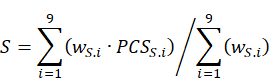
(5)
The Sustainability dimension performance class is assessed considering the dimension score and the dimension thresholds, according to Figure 12.
Figure 12. Sustainability performance classes and thresholds.

Source: JRC.
[1] Building Research Establishment Environmental Assessment Method (BREEAM): https://breeam.com
[2] Institute for Innovation and Transparency of Procurements and Environmental Compatibility (ITACA) Protocol: https://www.proitaca.org/
[3] Leadership in Energy and Environmental Design (LEED): https://www.usgbc.org/leed
[4] Green Star: https://new.gbca.org.au/
[5] Comprehensive Assessment System for Built Environment Efficiency (CASBEE): https://www.ibecs.or.jp/CASBEE/english/
3.4 Minimise the use of fossil fuels in the built environment (S.1)
3.4.1 Description and assessment
At building scale, minimise the use of fossil fuels in the built environment (S.1) KPI is assessed through the following three indicators:
- Primary energy demand improvement (S.1.1).
- Optimisation of electricity peak demand for building operations (S.1.2).
- Smart readiness of buildings (S.1.3).
S.1 score at building scale is evaluated according to Equation (6) using different indicator weights (wS.1.j) depending on the different combinations of the project classification according to type (i.e. newbuild or renovation)/main use (i.e. residential or non-residential) of a building scale project, as reported in Table 5. As example, the indicator weights within Equation (6) refer to a project classified as building scale, newbuild type, and residential main use.
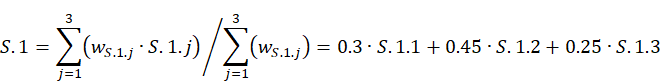
(6)
S.1 thresholds to associate the KPI score to the corresponding KPI performance class, at the building scale, are illustrated in Figure 13.
Figure 13. S.1 performance classes and thresholds at building scale.

Source: JRC
At neighbourhood/urban scale, Minimise the use of fossil fuels in the built environment (S.1) KPI is assessed through the following two indicators:
- Primary energy demand improvement (S.1.1).
- Smart energy meters (S.1.3).
The S.1.2 indicator, considered at building scale, is not applicable for the neighbourhood/urban scale projects. Accordingly, S.1.2 is omitted in the evaluation of S.1 score at neighbourhood/urban scale according to Equation (4) using different indicator weights (wS.1.j) depending on the different combinations of the project classification according to type (i.e. newbuild or renovation)/main use (i.e. residential or residential/non-residential) of a neighbourhood/urban project, as indicated in Table 5. It is worth noting that the denominator of Equation (4) equals unity for each combination. As example, the indicator weights within Equation (7) refer to a project classified as neighbourhood scale, renovation type and residential main use.
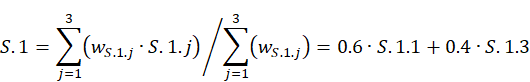
(7)
The S.1 thresholds to associate the KPI score to the corresponding KPI performance class at the neighbourhood/urban scale are illustrated in Figure 14.
Figure 14. S.1 performance classes and thresholds (neighbourhood/urban scale).

Source: JRC.
The S.1 KPI and its corresponding indicators can be generally implemented in the self-assessment of any project irrespective of its scale/type/main use. However, special attention should be drawn upon cultural heritage buildings since minimum requirements in relevant energy-related EU directive, e.g. the EPBD, may allow EU Member States to exclude this category of buildings from meeting NZEBs and/or zero-emissions building-targets in their national codes/regulations. Nevertheless, interventions to reduce the primary energy demand and the electricity peak demand can also be considered for historic buildings and heritage areas, carefully evaluating the feasibility of potential options case by case.
3.4.2 Primary energy demand (S.1.1)
At building scale, S.1.1 is evaluated based on the Level(s) indicator 1.1 for the primary energy demand (Dodd et al., 2020a), according to the following standards at international level: ISO 52000-1 (ISO, 2017a), ISO 52003-1 (ISO, 2017b), ISO 52010-1 (ISO, 2017c), ISO 52016-1 (ISO, 2017d), and ISO 52018-1 (ISO, 2017e). The indicator focuses on both the primary energy demand of the technical systems of the building and the efficiency of the building envelope, and the delivered energy demand that can subsequently be monitored using data from metering. Specifically, S.1.1 evaluates the annual primary energy demand for the use stage of a building scale project per internal useful floor area (expressed as kWh/m2). The primary energy demand is related to various energy carriers, delivered to the building and used in the form of electricity, heat and fuel, to satisfy the uses within the building. The delivered energy is generally the one metered by the utilities. Reporting is therefore disaggregated into the energy used for heating, cooling and dehumidification, ventilation, and humidification; hot water; and lighting (optional for residential buildings) according to ISO 52000-1 (ISO, 2017a). National bodies decide if energy consumption for lighting in residential buildings, as well as energy for other services (e.g., electrical appliances, cooking, industrial processes) in all types of buildings shall be included or not in the assessments. The primary energy use is based on primary energy factors per energy carrier, which are derived from national or regional annual weighted averages or a specific value for on-site production. At the design stage, the energy needs can be converted into primary energy by applying the relevant primary energy factors. These factors account for any system losses and inefficiencies.
Energy can be imported or exported from/to the building from on-site, nearby, and distant energy generators. Inside the assessment boundary, primary energy factors shall apply to all forms of energy generation that supply the delivered energy needs of the building, as well as any exports.
For new buildings the indicator is estimated, while for existing buildings it is more appropriate to use metered data.
S.1.1 score is evaluated according to four-step framework, as follows:
Annual delivered energy demand sub-metric evaluation: the annual delivered energy is also referred to as annual final energy consumption. The energy is expressed per energy carrier, supplied to the technical building systems through the assessment boundary, thus delivered to the building in the form of electricity, heat and fuel to satisfy the building services according to ISO 52000-1 (ISO, 2017a). Specifically, the delivered energy for all building services included in the energy performance assessment is used for heating, cooling and dehumidification, ventilation, and humidification; hot water; and lighting (optional for residential buildings) according to ISO 52000-1 (ISO, 2017a). Additional building services can be integrated depending on the use of the building (e.g. hospitals, retail, etc.) and shall be reported separately. The evaluation can be carried out differently depending on newbuild or renovation projects, as follows:
a) Newbuild projects, the assessment first estimates the energy needs of the building and then considers the efficiency of different technologies to quantify the delivered energy demand. Electricity loads associated with occupancy, for example, plug loads for appliances or computers, are not specifically covered in most national or regional assessments. This effectively means that these are unregulated energy needs and they are reported separately if they are estimated.
b) Renovation projects (existing buildings), the delivered energy can be measured directly from the meters and the utility (energy) bills.
The annual delivered energy demand per energy carrier can be quantified according to standardised procedures. The starting point for estimating the delivered energy demand is the thermal performance of the building envelope (energy need), while the main input data items and available resources include: conditions of use and occupancy: ISO 52000-1 (ISO, 2017a), EN ISO 52016-1 (ISO, 2017d); thermal envelope description: ISO 52016-1 (ISO, 2017d); building services description: ISO 52016-1 (ISO, 2017d); reference year climate file: three climate zones (EN 15265 test cases); primary energy factors: EN 52000-1, Annex B.10 (ISO, 2017a); internal temperature set points: ISO 52016-1 (ISO, 2017d); ventilation and infiltration rates: EN 15241, EN 15242; internal gains as heat flows: ISO 52016-1 (ISO, 2017d).
The annual delivered energy demand can be assessed according to the following approaches:
- Building scale simulation tools that have been validated according to available standardised procedures (ISO, 2017d, ASHRAE 2023b), should be used to perform the assessment, e.g. DOE2, BLAST, ESP, SRES/SUN (SERIRES/SUNCODE), SERIRES, S3PAS (LIDER/CALENER), TAS, TRNSYS, EnergyPlus, among many others. Setting up a simulation model may be time-consuming, as it requires detailed inputs about a building. It is also recommended to assess the local climate. A good example is the tool Climate Consultant or collecting the data from the International Weather for Energy Calculation (IWEC) and use weather files for a Typical Meteorological Year (TMY) according to standardised climatic data (ISO, 2005).
Measured data for existing buildings can be used to quantify the delivered energy demand per energy carrier. Take the average over several most recent full years, as long as the building and its use pattern have been the same. If the period is shorter than three years, a weather correction shall be performed (ISO, 2017a).
a) Data for the delivered energy can be obtained from energy bills issued by service providers/utilities (e.g. electricity, natural gas).
b) Measured data shall be obtained from meters and sub-meters, or from a building energy management system (BEMS), if available. The amounts of all energy carriers delivered to the building and exported by the building shall be measured and reported.
c) Estimated annual amounts of fuels can be used if these are not automatically metered (e.g. liquid and solid fuels as oil or coal).
When dealing with utility bill data, for example, electricity from the main meter or natural gas used for space heating and cooking, the values represent the total energy demand of the building, making it challenging to reconstruct energy consumption for specific end uses. In case that the only source for measured data are utility bills, then it is necessary to have an end-use breakdown for the default building services.
For electricity, the available approaches include:
- Option 1 - utilise the statistical electricity profiles from national studies and databases (Odysee-Mure Data Tools, Eurostat Data Browser) that provide electrical energy consumption profiles for each end-use.
- Option 2 - list every electrical device, estimate how often it is used on annual basis and estimate its annual energy use using its technical specifications.
- Option 3 - use assessment methods and calibrate the results with measured data from the utility bills. Simulation tools can also be used to generate end-use breakdown.
For fuels, when the energy carrier is used for heating, cooking, and domestic hot water (DHW), the available approaches include:
- Option 1 - determine the baseloads by separately analysing seasonal consumption (winter and summer) to differentiate space heating from cooking and DHW; estimate DHW consumption depending on floor area or per person in the building using national statistics or European tools (TABULA web tool) and databases (Eurostat Data Browser); estimate consumption for cooking.
- Option 2 - assess the thermal delivered energy demand based on standards and calibrate the measured data with simulations to obtain the end-use breakdown.
Measured data should be normalised, according to ISO 52100-1 (ISO, 2017a), to account for:
- Weather: correction from actual to standard weather conditions; may use long time periods (e.g. average three-year data) or use the common practice for correcting with average heating degree days (HDD) and cooling degree days (CDD) from (Eurostat Degree Days).
- Occupancy and operation: correction from the actual to the standard occupancy pattern; occupancy profiles are used according to EN 16798-1 (CEN, 2019) (ANNEX A8), ISO 52000-1:2017 (ISO, 2017a), ISO 52016-1:2017 (ISO, 2017d), ISO 16798-1 (ISO, 2019). For existing building, use building surveys to provide additional refinement and better understanding of occupancy patterns and user behaviour.
- Energy services: to include only the energy services that are accounted in the assessment; use estimated data to correct total measured energy data for all services
- Total annual delivered energy demand per useful floor area: quantify the annual delivered energy demand for the different energy carriers per useful floor area A_(use,sp) = useful internal floor area (m2) in kilowatt-hours (kWh/m2 per year). The ‘useful floor area’ means the area of the floor of a building needed as a parameter to quantify specific conditions of use that are expressed per unit of floor area and for the application of the simplifications and the zoning and (re)allocation rules (EPBD).
- Total annual primary energy demand per useful floor area (Ep,Ause,an) metric evaluation: the annual primary energy demand (Ep) is estimated by considering the delivered and exported (if any) energy per energy carrier, according to Equation (8). Specifically, the delivered energy demand for each energy carrier (Edel,i) is multiplied with the corresponding regional-national primary energy factors (PEF) to convert to primary energy. The results can be disaggregated in non-renewable and renewable components and it is recommended to use national PEF values, especially for electricity (Amann et al., 2023). Several approaches/methods to determine the PEFs are indicated in the European standard EN 17423 (CEN, 2020). However, default PEF, if necessary, for on-site, nearby, or distant energy sources are available from ISO 52000-1 (ISO, 2017a) and RED (European (EU) 2023).
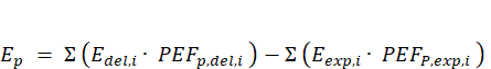
(8)
where Edel,i is the delivered energy for energy carrier i, Eexp,i is the exported energy for energy carrier i, PEFP,del,i is the primary energy factor for the delivered energy carrier i, ![]() is the primary energy factor for the exported energy carrier i.
is the primary energy factor for the exported energy carrier i.
The annual primary energy demand may be zero in case that on an annual basis the building may export as much energy it may be delivered to the building. This does not mean that there is no energy crossing the building boundary, but on an annual basis, as much primary energy is generated and exported from the building using renewables (e.g. electricity from photovoltaics) as the amount of delivered primary energy. For net positive primary energy buildings, will get a negative value annual primary energy demand. This refers to the notion that on average over the year there is a surplus of exported energy. To account for this new era of high-performance buildings, the baselines used for the benchmarking will have to be adapted accordingly and interpret the indicators accordingly based on how much more primary energy is exported.
Normalise per unit floor area, the annual primary energy demand intensity is estimated using Equation (9).
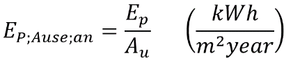
(9)
where Au = useful internal floor area (m2)
S.1.1 score evaluation: S.1.1 indicator is assessed using a performance scale (0, 100) between the baseline building and the national and local level target values for the zero-emissions buildings or the value for the NZEB building reduced by 10 %. The higher the value of the indicator, the better the performance towards the EU 2030 targets. The indicator could be measurable also at the EU level. The result is expressed as percentage of improved primary energy against a baseline reference at the local-national level or EU level. The indicator is assessed using Equation (10).
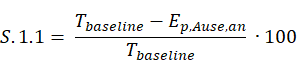

(10)
where Tbaseline = threshold assigned to the minimum value of the indicator which is the average of the annual primary energy demand of baseline building (kWh/m2 per year), EP;Ause;an= annual primary energy demand of the building (kWh/m2 per year)
A result greater than 32.5 % is considered positive in relation to the climate goal of reducing EU emissions by at least 32.5 % by 2030. This indicator allows us to track the progress towards the EU building stock by 2050. The maximum value of the indicator is 100. If the difference in the numerator is negative, i.e. the primary energy use intensity is below the reference baseline value, then the performance achieved is not sufficient and the value of the indicator is set to zero. Buildings should at least meet the minimum requirements for the primary energy demand.
The baseline building has an annual primary energy demand equal to the average annual energy primary of the reference building stock to which the building belongs (i.e. national or EU level). Depending on the building stock considered (national or EU-27), the primary energy demand of the baseline building will vary accordingly.
- The higher the value of the relative indicator, the better the performance of the building and the greater the reduction of primary energy demand.
- The relative values change from a minimum value of 0 (corresponding to the baseline reference) to a maximum value of 100 (corresponding to the zero-emission buildings target or the NZEB value reduced by 10 % for 2030).
- If the building performs as the baseline building, the value of the indicator would be 0.
Using the national baseline building, it is possible to assess the building performance in relation to the mean primary energy of the national building stock. Using the EU-27 baseline building, it is possible to assess the performance of the building in relation to the mean primary energy demand of the European building stock and the progress towards the EU 2030 and 2050 reduction targets. In the case of the EU-27 baseline building, a value of the relative indicator greater than 32.5 % is considered positive in relation to the EU 2030 reduction target.
The baseline value is not constant and is defined at national level, for different types of buildings. Using the EU baseline value, it is possible to assess performance of the building in relation to the EU 2030 and 2050 GHG reduction targets. Using a national baseline value, it is possible to assess performance of the building in relation to the national building stock. Several studies have investigated possible primary energy baselines and have proposed values to be used as benchmarks. However, there is no official standard or guideline. Following the EU policies in climate change mitigation, a well-accepted best practice for primary energy is the value that corresponds to an NZEB (see representative values in Table 6), which is defined by the EPBD. Member States have developed NZEB definitions in line with national, regional or local conditions in Table 7, including a numerical indicator of primary energy use (in kWh/m2y). According to the recast EPBD (Directive 2024/1275), Member States shall set the maximum national thresholds for the energy demand of a zero-emissions building at least the NZEB value reduced by 10 %.
If the assessment is performed at national level, the baseline value is the average annual primary energy demand of the national building stock. Relevant baselines may also be available from a statistical analysis of the primary energy reported in the energy performance certificates (EPCs). However, caution should be exercised when using these values to verify the different end-uses accounted for and the gap when compared against actual energy demand.
If the assessment is performed at EU level, the baseline value is the average annual primary energy demand of the EU building stock.
Table 6. NZEB reference baselines for residential and non-residential buildings.
| Climate zone | Building type | NZEBs Benchmark level | NZEB targets (kWh/m2.y) | |
| Net primary use (kWh/m2.y) | Total primary use (kWh/m2y) | |||
| Mediterranean (e.g., Catania, Athens, Larnaca, Luga, Seville, Palermo) | Residential Non-residential | 40-55 20-30 | 85-100 80-90 | 35-100 60-175 |
| Oceanic (e.g., Paris, Amsterdam, Berlin, Brussels, Copenhagen, | Residential Non-residential | 15-30 40-55 | 50-65 85-100 | 15-70 40-150 |
| Continental (e.g., Budapest, Bratislava, Ljubljana, Milan, Vienna) | Residential Non-residential | 20–40 40–55 | 50–70 85–100 | 20–125 25-125 |
| Nordic (e.g., Stockholm, Helsinki, Riga, Stockholm, Gdansk, Tovarene) | Residential Non-residential | 40–65 55–70 | 65–90 85–100 | 65–95 95–110 |
Source: Commission Recommendation, 2016.
The following best practices of EU-27 NZEB values for non-renewable annual primary energy average can be considered:
- New buildings: Residential: 59 kWh/m2; Non-residential: 79 kWh/m2.
- Existing buildings: Residential: 71 kWh/m2; Non-residential: 97 kWh/m2.
Table 7. NZEB energy performance levels in residential and non-residential, new and existing buildings in EU-27 Member States.
| EU Member State & UK | NEW BUILDINGS Non-renewable primary energy (kwh/ m2.y) | EXISTING BUILDINGS Non-renewable primary energy (kWh/m2.y) | Renewable Energy Sources | EPC | ||
| Residential | Non-residential | Residential | Non-residential | |||
| AT | 41 | 84 | 68 | |||
| BE-BRU | 45 | 85 | 55 | 100 | ||
| BE-FLA | 20 | 30 | 20 | 15 kWh/m2.y (residential), 20 kWh/m2.y (non-residential) | ||
| BE-WA | 85 | Relative requirement | A | |||
| BG | 43 | 63 | 43 | 63 | 55% | A+ |
| CY | 75 | 94 | 75 | 94 | 25% | A |
| CZ | 80 | 80 | ||||
| DE | 40 | 75 | 65 | |||
| DK | 37 | 51 | A 2015 | |||
| EE | 132 | 85 | 157 | 136 | Energy Class A-B (new residential), A (new non-residential), C (existing) | |
| EL | 37 | 92 | 75 | 138 | 15–60% depending on building type | A for new, B+ for existing |
| ES | 50 | 100 | A for new, B+ for existing | |||
| FI | 94 | 85 | 94 | 85 | B | |
| FR | 60 | 110 | 100 | 150 | ||
| HR | 28 | 21 | 28 | 21 | 30% | A+ |
| IE | 33 | 35 | 100 | 99 20% (new residential) A2 (new residential), A3 (new non- residential), B2 (existing residential) | 20% (new residential) | A2 (new residential), A3 (new non-residential), B2 (existing residential) |
| IT | 35 | 117 | 35 | 117 | 50% | |
| LT | 60 | 80 | 50% | A++ | ||
| LU | 45 | 60 | 45 | 60 | ||
| LV | 95 | 95 | 95 | 95 | A | |
| MT | 56 | 176 | 56 | 176 | 25% residential 20% non-residential | |
| NL | 30 | 28 | 30–50% | |||
| PL | 75 | 107.5 | 75 | 107.5 | ||
| PT | 35 | 130 | 55 | 140 | 50% (residential) A | |
| RO | 78 | 40 | 78 | 40 | 30% | |
| SE | 90 | 70 | A-C | |||
| SI | 70 | 55 | 95 | 65 | 50% | A1, A2, or B1 |
| SK | 54 | 61 | 54 | 61 | A0 | |
| UK | 45 | 150 | ||||
Source: D'Agostino et al., 2021.
At neighbourhood/urban scale, the assessment boundary of the indicator S.1.1 is for all buildings in the area. The assessment starts with quantifying the total delivered energy demand by estimating the annual final consumption of thermal energy and electrical energy for building operations for all buildings in the neighbourhood/urban project. This indicator quantifies the delivered energy demand for each building and then sums it up for all buildings. The total sum of delivered energy demand for all buildings in a specific area or city is then normalised with the number of “inhabitants and users” in that area. There are also numerous ways for modelling yearly supplied energy at the city scale. The primary energy demand is finally determined by converting the different energy carriers to primary energy. The indicator assesses the improvement in primary energy demand for all buildings over the national or local baseline average per capita.
Spatial energy modelling at city scale can be facilitated by Geographic Information System (GIS) especially for analysing, storing, managing, and visualizing big data using “top-down” (aggregate) and “bottom-up” (disaggregate) building energy models (Ali et al., 2021). For example (ISO, 2018), the total residential delivered electrical energy per capita shall be estimated as the total residential electricity use of a city in kilowatt-hours (numerator) divided by the total population of the city (denominator). The result shall be expressed as the total residential electricity use per capita in kilowatt hours/year. This may then be converted to primary energy demand, using the proper primary energy factor.
Repeat the assessment for all buildings in the neighbourhood-urban scale project. City-scale dynamic simulations are also available but are more complex, like the city-level dynamic energy simulation ( n.d.). Energy modelling approaches, for example, statistical regressions (Moghadam et al. 2018) and engineering archetypes (Moghadam et al. 2019) are applicable to model the final delivered energy demand for building stock.
Dealing with large scale urban environments, will encounter different types of buildings or mixed-use buildings, for which it may not be applicable to use the common indicator of energy per use floor area. In this case, it may be more appropriate to normalize the energy demand per capita, as follows:
- Residential buildings can use the number of inhabitants
- Tertiary buildings (e.g., gyms, swimming pools, museums, offices, hospitals) can use the number of users (customers, employees, hospital patients, visitors)
- Mixed residential and tertiary buildings can use the total number of inhabitants and users.
The normalization of the energy demand per capita at neighbourhood or city scale, can use the number of inhabitants of the city. The permanent population of a city is assessed according to ISO 37120 (ISO, 2018).
3.4.3 Electricity peak demand for buildings (S.1.2)
At building scale, the electricity peak demand (S.1.2) indicator measures the electricity peak demand reduction in a building during its use stage against a baseline reference, requiring as an input the hourly electricity demand (expressed in kW) from which to derive the maximum electricity demand.
For existing buildings, electricity power demand is commonly monitored on an hourly or quarterly basis for non-residential buildings and progressively for residential buildings as the installation of smart meters expands. It is increasingly becoming common to obtain this data from the records made available by the energy distributor.
For new buildings or during design, hourly energy simulations can be used to conduct in-depth and predictive analyses of electricity power demand. Through detailed modelling of building characteristics, energy systems, climatic conditions, and user behaviour, it is possible to accurately determine the peak electricity demand. These data are crucial for planning and designing appropriate electrical systems and ensuring that the building operates efficiently from an energy perspective. Additionally, they allow designers to properly size the required equipment and electrical supply to meet the building's demand.
The evaluation of the S.1.2 indicator is carried out by considering as assessment boundary the building and all areas of the building in which electricity is used for building operations. The S.1.2 score, which ranges between 0 and 100, is evaluated according to a three-step framework that consecutively estimate the scores of specific metrics to finally evaluate the indicator score, as follows:
Maximum electrical power (Ep,max) recorded in the year of operation metric evaluation: the hourly electric demand data of the examined building scale project needs to be analysed to determine the maximum electrical power in the year of analysis. Historical data demand for hourly electricity use may not be readily available, unless the building is equipped with a smart energy meter or a building management system. Alternatively, the maximum electrical power is indicated in the electricity contract and included in the utility bill, thus corresponding to the maximum power that can be supplied to the user. Relevant data can be obtained differently depending on newbuild or renovation projects, as follows:
a) Newbuild projects, use simulations to estimate the necessary data. Use these values to identify the maximum.
b) Renovation projects of existing buildings, these data can be obtained from the local energy distributor (as is the case in several European countries, e.g., Italy), typically provided at fifteen-minute intervals. Alternatively, the building must be equipped with smart meters that monitor instant electrical demand. In this case, the sum of the four measured values within the hour is used to obtain the energy (kWh) for that hour, and subsequently, power (kW).
Start from the hourly electric energy demand data recorded in the year of analysis to identify the maximum value for all building services included in the energy performance assessment.
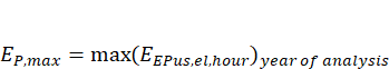 |
(11)
- Baseline (Tbaseline) metric evaluation: the evaluation carried out in step 1 needs to be repeated by using all historical hourly electrical demand data that precede the year of analysis considered in step 1, to identify the maximum electrical power (expressed in kW) from the historical data, according to Equation (12). In case these data are not available or relate to a historical period of less than one year, the baseline metric score corresponds to the maximum electrical power peak indicated in the electricity contract and included in the utility bill. This value corresponds to the maximum electrical power (EP,max) that can be supplied to the building.
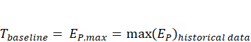 |
(12)
- S.1.2 score evaluation: the S.1.2 score is estimated according to Equation (13), as a ratio in which the numerator is obtained by subtracting the score of the EP,maxmetric (evaluated in step 1) from the score of the baseline metric (evaluated in step 2) and the denominator is the score of the same the baseline metric. The ratio is multiplied by 100, so that the indicator score can be expressed as a dimensionless value that varies between 0 and 100.
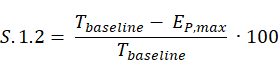 |
(13)
- The S.1.2 score indicates the extent to which the peak electricity demand recorded in the year of analysis varied from the baseline metric score. If the Ep,max metric score is lower than the baseline metric score, S.1.2 results into a positive score, noting though that the maximum indicator score is 100. The higher the indicator positive score, the better the performance achieved, indicating a more significant reduction of the annual peak power demand than historical peaks. If the Ep,maxmetric score exceeds the baseline metric score, leading the difference in the numerator to be negative, S.1.2 then the performance achieved is not sufficient and the value of the indicator is set to zero. Buildings should at least meet the minimum requirements for peak power demand.
- The Tbaseline scores to be used in Equation (13) as baselines for peak electricity demand in buildings across Europe vary depending on national regulations, climate, and the use of electrical equipment and appliances. The variability in electricity demand among countries and within the same country makes challenging to establish relevant baselines. Each building should refer to its specific case and requirements when determining its peak electricity demand. The Tbaseline scores may vary depending on the specific contractual agreements with local utilities, building characteristics, and user requirements, especially for non-residential buildings, as reported in the following for Italy, Germany, and France: In Italy, the average maximum contractual peak is typically 3 kW, with the potential to increase to 6 kW in larger or high-demand residences.
- In Germany, the average maximum contractual peak is typically 3.7 kW (16 Amperes at 230 Volts), but it can be adjusted according to consumer needs.
- In France, residential buildings are typically supplied with 9 kVA, approximately equivalent to 9 kW.
At neighbourhood/urban scale, the electricity peak demand (S.1.2) indicator is not used.
3.4.4 Smart readiness (building scale) or smart energy meters (neighbourhood/urban scale) (S.1.3)
At building scale, the assessment is based on the Smart Readiness Indicator (SRI) developed by the European Commission. The value of this indicator changes from 0 (corresponding to the baseline reference) to 100 (e.g. corresponding to the targets for 2030). The higher the value of the indicator, the greater the “smartness” of the building.
For each technical domain and impact criterion an EU-wide analysis was conducted to assess the maximum smartness functionality that is currently available on the market, the lowest level of smartness (usually no smartness at all), and the intermediate levels, as follows:
- If a technical domain in a building has the maximum smartness functionality for the given impact, the score is 100 % for the given impact criterion for that domain. There are nine technical domains including: heating, domestic hot water, cooling, ventilation, lighting, electricity, dynamic building envelope, electric vehicle charging, and monitoring and control.
- If there is no smart capability the score is set at 0 and can be used as a baseline
- Intermediate levels of smartness have intermediate values ranging between 0 and 100 (the maximum achievable).
However, not all technical domains contribute equally to any given impact criterion, so internally SRI the corresponding performance based on the relative importance of the domain to the impact criterion (as set out in Annex V of EPBD). For example, as space heating is typically around 65 % of total building energy consumption then its contribution to the overall energy efficiency score would be adapted to reflect its importance, while technical domains that make a smaller contribution would have smaller impact that is proportional to their contribution.
SRI does not account for the possible unique characteristics and limitations of cultural heritage buildings.
At neighbourhood/urban scale, the indicator considers the “percentage of buildings in the city with smart energy meters (%)” according to ISO 37122 (ISO, 2019).
The percentage of buildings in the city with smart energy meters shall be assessed as the number of buildings in the city with smart energy meters (numerator) divided by the total number of buildings in the city (denominator). The result shall be multiplied by 100 and expressed as the percentage of buildings in the city with smart energy meters.
At building scale, the assessment follows the Commission Delegated Regulation (EU) 2020/2155 for the smart-ready services that are present or planned at the design stage, and on their functionality level. They are listed in a pre-defined smart-ready service catalogue that is used by experts as the basis for identifying and assessing smart-ready features and is organized into nine pre-defined technical domains (Figure 15).
The assessment may follow:
- Method A - Simplified method, suitable for existing buildings or small non-residential buildings with low complexity. Use a simplified service catalogue that includes only 27 pre-defined services;
- Method B - Detailed method, suitable for new buildings and non-residential buildings that have a higher complexity. Use a detailed service catalogue that includes 54 pre-defined services;
Figure 15. Overall structure of the Smart Readiness Indicator (SRI) service catalogue.
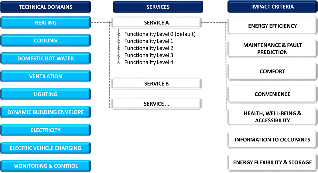
Source: Adapted from Verbeke et al., 2020.
The assessment steps include:
- Select services for each domain: the SRI rating depends on the examined building’s ability to facilitate “smart-ready” services which are included in a “smart-ready service catalogue”, addressing nine technical domains: (1) heating (2) domestic hot water; (3) cooling; (4) ventilation; (5) lighting; (6) dynamic building envelope; (7) electricity; (8) electric vehicle charging; and (9) monitoring and control. The full catalogue of SRI smart ready services contains a list of 54 services.
- Assess functionalities: For each service, 2 to 5 functionality levels are defined. A higher functionality level reflects a “smarter” implementation of the service, which generally provides more beneficial impacts to building users or to the grid compared to services implemented at a lower functionality level. The functionality levels are expressed as ordinal numbers, implying that ranks cannot be readily compared quantitatively from one service to another.
- Impact score: The total smart readiness score of a building is a percentage that expresses how close (or far) the building is to maximal smart readiness. The higher the percentage is, the smarter the building.The SRI score is based on a weighted sum of the 7 total impact scores. In this multi criteria assessment, the weighting factors can be attributed to both domains and impact criteria to reflect their relative contributions to an aggregated overall impact score. A total SR score indicates the overall smartness level of the building, while sub-scores allow to assess specific domains and impact categories.
- Smart readiness score evaluation: the total smart readiness score SR may be assessed, as a weighted sum of the key functionalities’ smart readiness scores, using Equation (14).
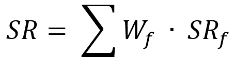
(14)
where SRf is the smart readiness score for key functionality f, Wf is the weight of key functionality f in the estimation of the total smart readiness scores, with ΣWf = 1.
The smart readiness scores of technical domains for each impact criterion SRd,ic are estimated according to Equation (15).
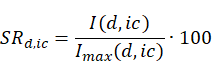
(15)
where I(d,ic) is the score of domain number d for impact criterion ic, Imax(d,ic) is the maximum score of domain number d for impact criterion number ic.
5. S.1.3 score evaluation: the indicator is assessed using Equation (16).
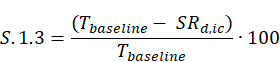
(16)
where SRd,ic = Total SR score (%), Tbaseline = threshold assigned to the value minimum of the indicator which is the baseline building value (%).
The evaluation of a building is facilitated with an Excel-based tool. More details are also available in the SRI training slides (SRI Implementation tools n.d.).
If the value of the metric is greater than the reference baseline value, the achieved performance is positive and the indicator value can be considered in the KPI assessment. The maximum value of the indicator is 100. If the difference in the numerator is negative, i.e. the building’s SRI is below the reference baseline value, then the performance achieved is not sufficient and the value of the indicator is set to zero. Buildings should at least meet the minimum requirements for smart readiness indicator.
Detailed field data is not yet widely available to derive representative SRI scores, since the SR is currently emerging. As example, from a small set of buildings, SRI scores from five countries and for the different scenarios and methods are summarized in Table 8. The study was designed to evaluate the retrofitting cost towards smartification for typical residential buildings. Initially the SR was estimated for a baseline scenario, i.e. the status of typical residential buildings, and then for two consecutive cycles of retrofitting towards smartification scenarios (Scenario A and Scenario B) aiming to increase the buildings’ energy performance but mainly its smartness considering plug-and-play, cost efficient interventions.
Table 8. Total SRI scores and SRI class for different scenarios and methods.
| Total SRI score (%) – SRI class (A-G) | Baseline | Scenario A | Scenario B | |||
| Method A | Method B | Method A | Method B | Method A | Method B | |
| Single-Family Houses | ||||||
| Denmark | 7% (G) | 7% (G) | 37% (E) | 32% (F) | 70% (C) | 68% (C) |
| Czech Republic | 8% (G) | 4% (G) | 33% (F) | 27% (F) | 70% (C) | 66% (C) |
| Greece | 16% (G) | 9% (G) | 41% (E) | 31% (F) | 73% (C) | 69% (C) |
| Bulgaria | 4% (G) | 2% (G) | 28% (F) | 26% (F) | 66% (C) | 64% (D) |
| Austria | 5% (G) | 4% (G) | 29% (F) | 23% (F) | 68% (C) | 67% (C) |
| Av. score (SFH) | 8% | 5% | 34% | 28% | 70% | 67% |
| Multi-Family Houses | ||||||
| Denmark | 8% (G) | 30% (F) | 65% (C) | |||
| Czech Republic | 4% (G) | 27% (F) | 65% (C) | |||
| Greece | 12% (G) | 30% (F) | 65% (C) | |||
| Bulgaria | 5% (G) | 24% (F) | 60% (D) | |||
| Austria | 5% (G) | 27% (F) | 69% (C) | |||
| Av. score (MFH) | 7% | 28% | 65% | |||
Source: Apostolopoulos et al., 2022.
The baseline scenario represents buildings with the national minimum requirements in terms of energy performance (according to the relevant national EPBD legislation). Buildings constructed after 2010 are considered energy efficient and thus the proposed retrofitting scenarios are limited to active systems without considering renovation of the building envelope. Scenario A considers market available technologies to help buildings move towards NZEB and Scenario B integrates more technologies that move past NZEB that can contribute to classifying the buildings as PEBs. According to results, the minimum national requirements in compliance with EPBD requirements for single-family houses lead to an average SRI score of 8 % and 5 % for Method A and B respectively. For MFH, the average is 7 % for Method B. The SRI assessment of the baseline status led to scores that range from 2 % to 9 % for single-family and from 4 % to 12 % for multi-family houses.
At neighbourhood/urban scale, a different indicator is used. According to ISO 37122 (ISO, 2019) the percentage of buildings in the area with smart energy meters shall be assessed as the number of buildings in the area (Nsm) with smart energy meters (numerator) to the total number of buildings (Nt) in the area (denominator). The result shall be multiplied by 100 and expressed as the percentage of buildings in the city with smart energy meters.
The update and progress with smart energy meters has been slow in the EU-27, despite the legislative and regulatory frameworks that have been in place for several years. Furthermore, the lack of harmonised standards for energy meters may create additional delays with the certification of the meters. Leading countries include Sweden, Finland, Spain and Estonia have been leading the effort, reaching 100 % deployment of automated smart meters, and in many cases are already replacing the old units with modern and more flexible meters. Other countries like France, Germany and Ireland, have recently initiated the rollout of smart energy meters. The target is to reach European coverage by 2030. Currently, the penetration level of energy smart meters (ESM) in the EU is estimated at 43% that can be used as an average EU-27 baseline (Tounquet and Alaton 2019).
The indicator is then assessed using Equation (12) as the difference of the result against the reference baseline value (Tbaseline) of the installed energy smart meters (numerator) divided by the baseline value of the energy smart meters in the area (denominator). The maximum value of the indicator is 100. S.1.3 can also be assessed against a baseline that is set at a value representing the existing status at the beginning of the project.
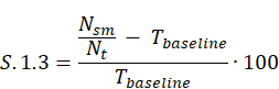
(12)
If the difference in the numerator is negative, then the performance achieved is not sufficient and the value of the indicator is set to zero. Cities should at least meet the minimum requirements for the penetration of smart energy meters to facilitate the electrification and decarbonisation efforts of the European building stock.
If the difference in the numerator is negative, then the performance achieved is not sufficient and the value of the indicator is set to zero. Cities should at least meet the minimum requirements for the penetration of smart energy meters to facilitate the electrification and decarbonisation efforts of the European building stock.
3.4.5 Example (S.1)
A new naturally ventilated multi-family residential building consisting of 22 dwellings for a useful internal floorarea equal to 2700 m2, located in Turin (Italy), is considered. The central space heating and domestic hot water (DHW) of the building are served by a natural gas fired non-condensing boiler, whereas the space cooling is served by local air-to-air heat pumps with indoor controls in each space. The metered annual energy consumption due to natural gas and electricity from the grid results into a value equal to 18351 m3 and 53 360 kWhe, respectively. The electricity use of a typical apartment within the building was monitored throughout 2022 and the hourly profile in Figure 16 corresponds to the week during which the electricity peak demand, equal to 3.2 kW, occurred, thus this value is considered representative to estimate the maximum electricity demand for the entire building.
Figure 16. Hourly profile of electricity demand for the example (S.1)
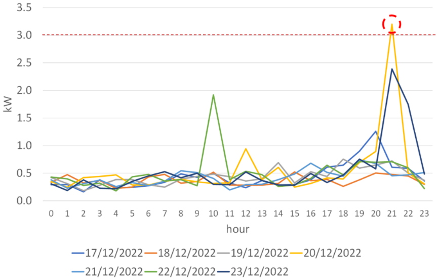
Source: JRC.
The evaluation of the S.1 KPI at building scale to minimise the use of fossil fuels in the built environment depends on the scores of S.1.1, S.1.2 and S.1.3 indicators.
The S.1.1 score is evaluated according to the four-step framework (Section 3.4.2) to estimate the scores of specific sub-metrics and metrics to finally evaluate the indicator score, as follows:
- Annual delivered energy demand metric evaluation: following ISO 52000-1:2017 (ISO, 2017a), the building services included in the assessment are: heating, cooling, ventilation, humidification, dehumidification, DHW. For this example, there is no mechanical ventilation and no dedicated humidification or dehumidification services. Following the breakdown of the total metered electricity according to EN 16247-2:2022 the specific building services from electricity (i.e. cooling) account for 6 % or 3,202 kWhe, while other uses like lighting, cooking, white appliances and plug loads account for 93 % or 50,158 kWhe.
The delivered energy with the metered quantity of natural gas is estimated as follows:
Efuel=Qfuel∙ LHV = 18,351∙ 9.45= 173,417 kWhth
where Qfuel = annual quantity of natural gas delivered to the building (m3), LHV = lower heating value of the natural gas (kWhth/m3).
The output of this step is to quantify the delivered energy per energy carrier allocated for the corresponding building services.
| Energy Carrier | kWh/year | Building services | Primary energy conversion factors |
| Natural gas | 173 427 | Heating, DHW | 1.05 |
| Electricity | 3 202 | Cooling | 2.42 (from Italian Ministry of Economic Development)[1] |
| Electricity | 50 158 | Other (i.e. lighting, cooking, white appliances, plug loads) |
[1] Supplemento ordinario alla “Gazzetta Ufficiale„ n. 162 del 15 luglio 2015 - Serie generale DECRETO 26 giugno 2015 N.39.
For information, if the available utility energy data include other end-uses that are not part of the considered services (e.g. use of natural gas for cooking, use electricity for appliances and lighting), then it will be necessary to estimate and allocate the energy for the different services. For example, use the energy bills during the off-heating season to determine the base loads for the use of natural gas for DHW and/or cooking, if that is applicable. This will be a first estimate, although there will be deviations on the energy use on an annual basis considering higher energy consumption for DHW in winter because of the lower water temperature.
Similar analysis must also be performed with the total electricity consumption from a utility meter to make the proper allocation of the total electricity to specific services considered in the methodological approach, i.e. exclude the energy used for lighting for residential buildings and appliances. The national household average annual consumption for appliances and lighting from the statistical analysis of Italian data provided by ENEA is 2072 kWhe. This data consists of the energy use by refrigerator 299.1 kWh/year, horizontal freezer 83.4 kWh/year, dishwasher 170.0 kWh/year, washing mashing 220.8 kWh/year, PC 91.8 kWh/year, TV 235.84 kWh/year, hair dryer 281.3 kWh/year, electric oven 198.2 kWh/year, iron 149.6 kWh/year, vacuum cleaner 163.9 kWh/year, (total of 1,888.8 kWh/year) and lighting (183.2 kWh/year).
- Total annual delivered energy demand per useful floor area metric evaluation: The normalized energy use intensity per unit floor area for the relevant building services is given as follows:
Natural gas: ![]()
Electricity: 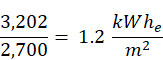
For information, the electricity consumption for the other building services is ![]()
- Total annual primary energy demand metric evaluation: The national primary energy factors for Italy are used to convert the final to primary energy demand as follows:
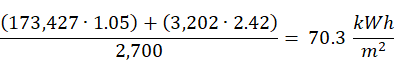
- S.1.1 score evaluation: the building is in climate zone E defined by the Italian decree on thermal energy systems (DPR, 412/1993) as shown below (A is warmest and F is coldest climate zone). The baseline of the primary energy demand for non-renewable is 221.1 kWh/m2.year
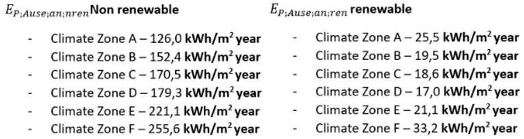
The value of the indicator for the primary energy demand for the specific building services becomes:
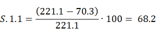
Discussion:
The NZEB target for non-renewable primary energy in Italy is 35 kWh/m2 and the best practice is equal to 22.3 kWh/m2 per year (mean statistical primary energy demand value for the higher energy class A4).
Apparently, there is room for improvement for the specific building, considering some additional energy efficiency measures to decrease the energy demand and use onsite renewables to cover some of the demand (see S2.1).
The S.1.2 score is evaluated according to the four-step framework (Section 3.4.3) to estimate the scores of specific metrics to finally evaluate the indicator score, as follows:
4. Maximum electric power (Ep,max) recorded in the year of operation metric evaluation: according to data on the hourly electricity demand recorded in the year of analysis (i.e. 2022) for a typical dwelling in the new building (Figure 16), the maximum electrical power for the representative dwelling is identified by using Equation (11), as follows (Equation (17))
(17)
Based on this score, it is possible to estimate the maximum electrical power for the entire building, considering that the total number of dwellings within the building is 22. Hence, the maximum electrical power for the building is estimated equal to70.4 kW.
5. Baseline metric evaluation: historical data are not available to estimate the baseline metric score, as the builing is new. Hence, the maximum electrical power in the electricity contract reported in the electricity bill is considered. Specifically, in Italy, the maximum peak for a dwelling in the electricity contract is typically 3 kW (red line in the demand profile identified in Figure 16) with the potential to increase to 6 kW in larger or high-demand dwellings. Based on this contractual data, the peak for the entire building ranges from 66 to 132 kW. The score of the baseline metric related to the entire building is estimated equal to the average of the aforementioned two values, thus being equal to 99kW.
6. S.1.2 score evaluation: based on the scores of EP,max (evaluated in step 1) and Tbaseline (evaluated in step 2), S.1.2 score is estimated using Equation (13), as follows (Equation (18)):
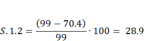 |
(18)
The S.1.2 indicator results into a positive score, thus indicating that the electricity peak demand of the building scale project analysed is lower than the baseline metric. However, a better score can be achieved if some improvement actions are considered. Examples in this direction refer to (i) increase user awareness but most importantly smart controls, that are critical in reducing the simultaneous use of high-consumption devices, (ii) enhance energy efficiency that is a priority and plays an important role for reducing peak electricity demand, among others for electrical appliances, equipment and other services, and (iii) in the context of building electrification, replacing gas-fired boilers and switching to heat pumps, or using induction plates for cooking, energy efficiency becomes crucial.
The S.1.3 score is evaluated according to the four-step framework (Section 3.4.4) to estimate the scores of specific metrics to finally evaluate the indicator score, as follows:
- Select services for each domain: Method A is usually sufficient for residential buildings. However, Method B that is mainly orientated for more complex non-residential buildings can be also used since it provides higher level information for the examined smart-ready services. The assessment used the default factors for the multicriteria evaluation.
A smart-ready service catalogue is available that contains a list of 54 potential services to address the domains of 1) Heating, 2) DHW, 3) Cooling, 4) Lighting, 5) Dynamic building envelope, 6) Electricity, and 7) Monitoring and control for the specific example. In general, can consider 9 domains, including Ventilation, and Electric vehicle charging. Some smart ready services for the specific example: heat emission control, control of DHW storage charging, cooling emission control, window solar shading control, reporting information regarding local electricity generation.
2. Assess functionalities: There are three key functionalities for the assessment. 1) optimise energy efficiency and overall in- use performance, addressing energy efficiency and maintenance & fault prediction; 2) adapt operation to the needs of the occupant, addressing comfort, convenience, health and well-being, and information to occupants; 3) adapt to signals from the grid (energy flexibility and storage).
3. Impact score: A total impact score is estimated for each impact criterion as a balanced impact sum for all the domain impact scores. The result is aggregated for the different impact categories for the three key functionalities.
4. Smart readiness score evaluation: The overall SRI score of the building is estimated at 12 %.
5. S.1.3 score evaluation: The SRI baseline is 8 % for multi-family apartment buildings, therefore the score of S.1.3 indicator is evaluated using Equation (16) and results equal to 71.4, according to Equation (19).
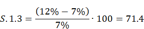 |
(19)
Discussion:
- Buildings that are constructed under the EPBD provisions, can increase smartness easier and at a relatively lower cost than older buildings (Apostolopoulos et al. 2022).
- On average, buildings perform better in “Health, well-being and accessibility” and “Comfort” impact categories.
- Emphasis on improving the building’s smartness like building automation and control measures can increase can improve the overall performance to (65–80%) and perform better in improving energy efficiency towards NZEB.
- More emphasis should be given to solutions that could support interaction with the grid, especially considering the integration of renewables (S.2.1) and storage (S.2.2), towards energy net positive buildings.
Having evaluated the scores of S.1.1 and S.1.2 indicators, S.1 is evaluated by using Equation (6) and considering the indicator weights corresponding to the combination of the project classification as building scale, newbuild type, and residential main use (Table 5). Hence, S.1 results into a score estimated equal to 51.3 that corresponds to the Good performance class (Figure 13), as reported in Table 9. S.1 score can be increased to attain the Excellent class Based on the results of the indicator scores, placing more emphasis on reducing the electricity peak load can help enhancing S.1 score, considering the relatively low score of the indicator and the relatively high indicator weight. This is understandable considering the importance that peak electricity demand will play as buildings move to the electrification era, mandating very careful consideration of loads on the grid.
Table 9. Example of S.1 evaluation (building scale).
| Indicator | S.1.1 | S.1.2 | S.1.3 |
| Indicator score | 51.5 | 28.9 | 71.4 |
| S.1 score | 0.3 • 68.2 + 0.45 • 28.9 + 0.25 • 71.4 = 51.3 | ||
| S.1 performance class | Good | ||
| S.1 performance class score (PCSS.1) | 70 | ||
Source: JRC.
The neighbourhood/urban scale project considers that the penetration of smart energy meters in the area has been very good and stands at 81 %.
— Assess S1.1 – Primary energy demand
Repeat the assessment for all buildings in the area, following similar steps as in the building scale. The area will include residential and non-residential buildings. The value of the indicator following a large scale renovation project is estimated at 74 %.
— Assess S.1.3 – Smart energy meters
The area has advanced with the installation of smart energy meters that currently stands at 81 %, which is high compared to the EU baseline at 43 %.
The value of the relative indicator then becomes:
The KPI then becomes for the renovation project:
S.1 = 74 • (0.55) + 88.4 • (0.45) = 89.3
The result for the KPI performance class is “Excellent” since it exceeds the threshold value of 75.
3.5 Maximise the use of sustainable energy in the built environment (S.2)
3.5.1 Description and assessment
At building scale, maximise the use of sustainable energy in the built environment (S.2) KPI is assessed through the following two indicators:
- Share of renewables (S.2.1).
- Energy storage (S.2.2).
S.2 score at building scale is evaluated according to Equation (20) using different indicator weights (wS.2.j) depending on the different combinations of the project classification according to type (i.e. newbuild or renovation)/main use (i.e. residential or non-residential) of a building scale project, as reported in Table 5. As example, the indicator weights within Equation (20) correspond to the combination of the project classification according to scale/type/use into building, newbuild, and residential, respectively.
(20)
The S.2 thresholds to associate the KPI score to the KPI performance class, atbuilding scale, are illustrated in Figure 17, differentiating by building type/main use.
Figure 17. S.2 performance classes and thresholds (building scale).

Source: JRC
At neighbourhood or urban scale, maximise the use of sustainable energy in the built environment (S.2) KPI is assessed thorugh the same two indicators considered at building scale. S.2 score at neighbourhood/urban scale is evaluated according to Equation (21) using different indicator weights (wS.2.j) corresponding to the different combinations of the project classification according to type (i.e. newbuild or renovation)/main use (i.e. residential or residential/non-residential) of a neighbourhood/urban scale project, as reported in Table 5. As example, the indicator weights within Equation (21) correspond to the combination of the project classification according to scale, type, and use into building, renovation, and residential, respectively.
(21)
The S.2 thresholds to associate the KPI score to the KPI performance class, at neighbourhood or urban scale, are illustrated in Figure 18.
Figure 18. S.2 performance classes and threshols (neighbourhood and urban scale).

Source: JRC
The S.2 KPI and its two corresponding indicators can be generally implemented in the self-assessment of any project irrespective of its scale/type/use. However, the building‑integration of energy systems based on renewable sources should carefully consider the aesthetic aspects of a building project and preserve its architectural features. Special care should also be exercised with cultural heritage buildings since minimum requirements in relevant energy-related EU directive like EPBD may allow EU Member States to exclude cultural heritage from the use of renewables in their national codes/regulations. Nevertheless, opportunities and technology solutions to properly integrate renewables in historic buildings and heritage areas (e.g. Roman-style photovoltaic roof tiles) can also be considered, carefully evaluating the feasibility of potential interventions case by case.
3.5.2 Share of renewables (S.2.1)
At building scale, the S.2.1 indicator is assessed based on Level(s) indicator 1.1 (Dodd et al., 2020a) to take into account the benefits of generating renewable energy to satisfy the primary energy demand, according to the following standards at international level: ISO 52000-1 (ISO, 2017a), ISO 52003-1 (ISO, 2017b), ISO 52010-1 (ISO, 2017c), ISO 52016-1 (ISO, 2017d), and ISO 52018-1 (ISO, 2017e). The indicator takes into account both the building thermal and electrical delivered energy demand, as well as the quantity of generated thermal and electrical energy from renewable sources. The delivered energy demand can be monitored using metered data, common for existing buildings to be renovated, or estimated data, common for new buildings.
The evaluation identifies the percentage of renewable energy sources within the comprehensive energy mixture, covering both thermal and electrical components (on-site, nearby, and distant) according to ISO 52000-1(ISO, 2017a), as illustrated in Figure 19.
Figure 19. Schematic concept of assessment boundaries
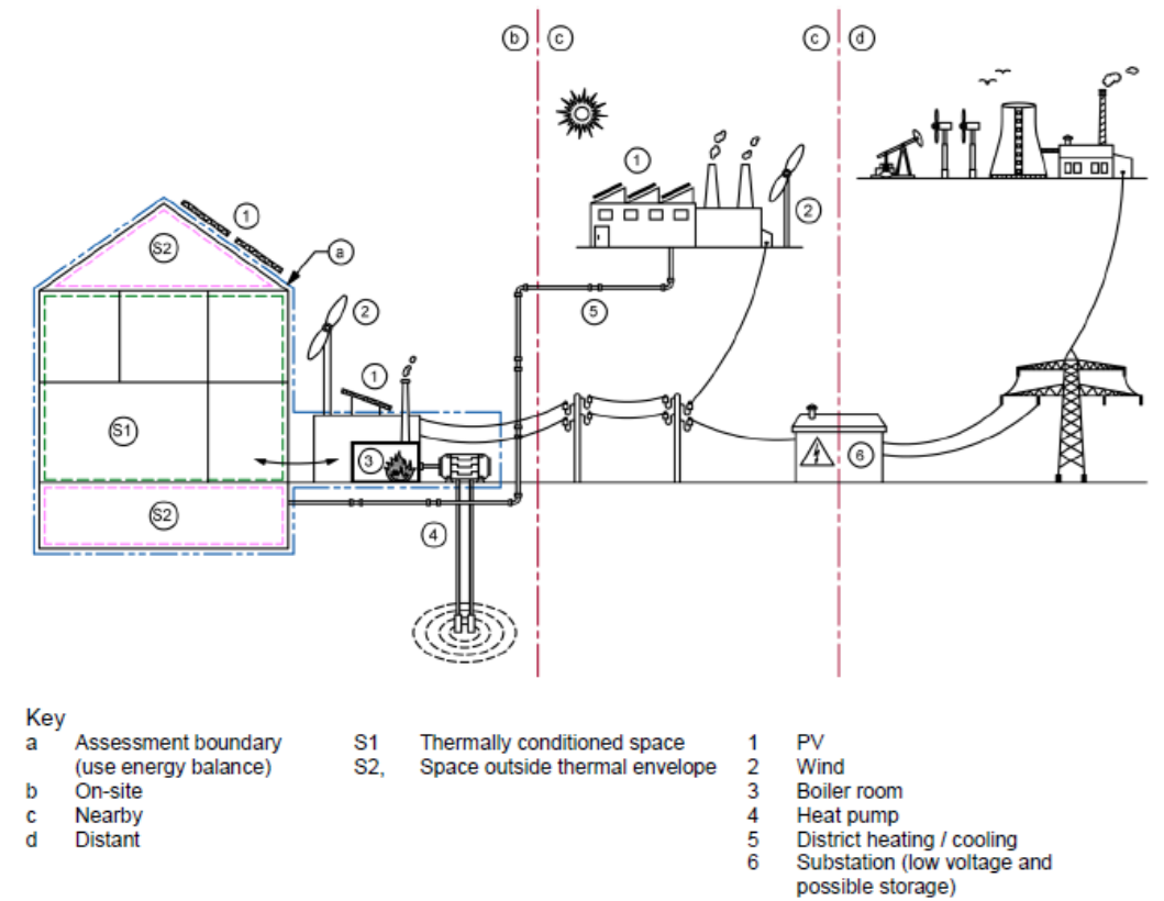
Source: Dodd et al. 2020a.
The underlying assessment method is based on ISO 52000-1 (ISO, 2017a) and ISO 52016-3 (ISO, 2023). Procedures on the energy from renewable energy sources related to different technologies (thermal solar systems, heat pumps, etc.) are given in the related sub-system EPBD standards.
The building assessment boundary includes all areas of the building in which useful thermal energy or electricity is used or produced. This boundary may not coincide with the physical boundary of the building (e.g., if a part of the technological system is located outside the building but constitutes part of the energy uses considered, it is considered included in the assessment boundary of the building).
The S.2.1 score, which ranges between 0 and 100, is assessed according to a four-step framework that consecutively estimates the scores of specifc sub-metrics and metrics to finally evaluate the indicator score, as follows:
- Annual delivered energy demand (Ec for electricity and Qc for thermal energy) sub-metric evaluation: the annual delivered energy demand (for all forms of energy expressed in kWh/year) is evaluated according to the same procedure indicated in the step 1 for the evaluation of the S.1.1 indicator (Section 3.4.2): (i) on-site energy (Ep for electricity and Qp for thermal energy), that is the energy produced by on-site plants, (ii) exported energy (Ee for electricity and Qe for thermal energy), that is the share of energy produced on-site and not used, thus exported for each renewable energy generator, and (iii) imported energy (Ei for electricity and Qi for thermal energy), that is the amount of energy from renewable sources delivered by distant/nearby generators into the assessment boundary, e.g. district heating, electricity grid.. Estimated energy data are preferable for new buildings, while metered energy data are more appropriate for existing buildings to be renovated.
Annual delivered energy demand for building operations covered by renewable energy sources (ERES for electricity and QRES for thermal energy) sub-metric evaluation: all renewable energy [1] generators within the assessment boundary need to be identified to subsequently determine the three main shares of energy (expressed in kWh/year) for electrical and thermal energy: (i) on-site energy (Ep for electricity and Qp for thermal energy), that is the energy produced by on-site plants, (ii) exported energy (Ee for electricity and Qe for thermal energy), that is the share of energy produced on-site and not used, thus exported for each renewable energy generator, and (iii) imported energy (Ei for electricity and Qi for thermal energy), that is the amount of energy from renewable sources delivered by distant/nearby generators into the assessment boundary, e.g. district heating, electricity grid. Subsequently, add the difference between the energy produced (on-site) and exported (nearby and distant) to the delivered energy by nearby/distant renewable generators (imported). The result is the annual total delivered energy demand for building operations from renewable energy sources. Similarly to the step 1, estimated energy data are preferable for newbuild projects, whereas metered energy data are more appropriate for renovation projects of existing buildings, as follows:
a) Newbuild project: energy flows need to be estimated by quantifying (i) the annual renewable energy by on-site generation components (i.e. on-site energy flows); and (ii) the annual delivered energy from nearby and distant energy renewable generators (i.e. imported energy flows), according to ISO 52000-1 (ISO, 2017a).
Regarding the on-site energy flows, the annual on-site renewable energy production for generated electrical and thermal energy from PV, wind, CHP and others is estimated, according to EN 15316-4-3 (CEN, 2017a). The assessment considers the time mismatch between the production and use of electricity (see Table B.32 in ISO 52000-1:2017 (ISO, 2017a)) to account for the time lag between electricity production and use and facilitates the breakdown of energy demand from renewable sources.
Regarding the imported energy flows, the imported electrical and thermal energy produced from all renewable sources may account from nearby and distant production sites for the specific building services. However, according to ISO 52000-1 (ISO, 2017a), the energy produced at a distant location and delivered to the building should not be considered in the renewable energy count. On the other hand, it is imperative to account for remotely generated renewable energy due to the growth of large-scale renewable installations, e.g. wind and photovoltaics, alongside the emergence of distributed renewable installations and local energy communities.
b) Renovation project: energy flows need to be measured by quantifying the annual renewable energy using actual operating data from (i) the total annual energy imported (electricity and heat bills) (i.e. imported energy flows), and (ii) the total annual energy produced by all on-site generators (i.e. on-site energy flows) reduced by the annual energy that is not used at the building site (i.e. exported energy flows). When data are extracted from energy bills, the method of energy demand breakdown is detailed in S.1.1.
As a result of the time mismatch between renewable energy production and building energy demand there is a need to support the installations with electrical and thermal energy storage (also refer to S.1.2). According to ISO 52000-1 (ISO, 2017a), the storage-weighted contribution is accounted as an auxiliary and it is added to the generator-weighted energy. Given that thermal and electrical storage systems are primarily powered by renewable energy sources during the charging phase, it is reasonable to consider the energy released by these systems as a contribution to renewable energy. This feature makes them significant contributors to clean energy when providing power in response to demand.
Using an energy storage system onsite, can reduce the exported energy from the building that is stored and used at a later time, thus reducing the imported energy. Estimated energy storage is preferable for newbuild projects, whereas measured energy storage is more appropriate for renovation projects of existing buildings, as follows:
a) Newbuild project: energy storage need to be estimated, thus the storage can be considered a common sub-system. The energy delivered to the building for heating use is obtained according to EN 15316–5 (CEN, 2017b), whereas the energy delivered to the building for cooling is estimated according to EN 16798-15 (CEN, 2017c) and EN 16798-16 (CEN, 2017d). The energy delivered by the storage systems is estimated as follows: define the initial state of charge of the storage (in the case of thermal storage this means the temperature level); quantify the energy stored by the storage unit; quantify the energy supplied; state of charge of the storage after discharge; energy required for charging; energy losses.
b) Renovation project: Measure energy storage: Energy flows are monitored and tracked, in order to quantify the energy delivered and used for building services, whether this energy is from onsite renewables production and direct use or from storage.
- Renewable energy (REStot) metric evaluation: the REStot metric evaluates the share of renewable energy to the annual total delivered energy demand for building operations. The metric is estimated as the ratio of the annual total delivered energy demand (including both electricity and thermal energy) for building operations covered by renewable energy sources (ERES) (evaluated in step 2) to the annual total delivered electricity and thermal energy demand (EP) (estimated in step 1), expressed as a percentage, according to Equation (22). The greater the metric score, a more sustainable total energy use; thus indicating a more environemental-friendly building that exhibits less dependency on non-renewable energy sources. Despite a high share of renewable energy, the energy efficiency and a lower energy demand of a building scale project remain key-priorities to ensure no energy-related waste.
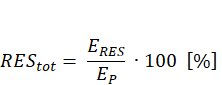
(22)
4. S.2.1 score evaluation: S.2.1 score is estimated according to Equation (23), as a ratio in which the numerator is the difference of the REStotmetric score (evaluated in step 3) against the score of a baseline metric (Tbaseline) at the local/national or EU level, and the denominator is the score of the same baseline metric, multiplied by 100, so that the indicator score can be expressed as a dimensionless value that varies between 0 and 100. The score of the baseline metric corresponds to the average share of renewable energy on the total final energy consumption (i.e. electricity, heating and cooling) of the national or EU building stock to which the building scale project belongs.
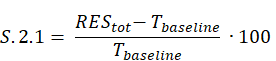
(23)
If the REStotmetric score is greater than the Tbaselinemetric score, S.2.1 results into a positive score that may also exceed 100 in the event of a net positive building, noting though that the maximum indictor score is set to 100. If REStotmetric score is lower than the Tbaselinemetric score, leading the difference in the numerator to be negative, S.2.1 results into a negative score indicating that the performance achieved does not satisty the baseline metric due to a lower proportion of renewbale enrgy integration and the indicator score is set to zero (0). Furthermore, when the REStotmetric score is equal to zero, the building is completely supplied by fossil fuel. Buildings should at least meet the minimum requirements for the share of renewables. The score of the baseline metric to be used in Equation (23) varies depending on the national or EU context considered, although the share of renewable energy on the total final energy consumption (i.e. electricity, heating and cooling) of the national or EU building stock is not immediately provided in available databases or standards. At EU level, the current practice for the share of renewables on the final energy consumption for three sectors (i.e. transport, electricity, and heating and cooling) in EU-27 Member States is available from Eurostat (2023b), accounting for an EU average share of energy consumption from renewables for electricity generation and for heating and cooling in 2022 equal to about 41.2 % and 24.8 %, respectively. These data may be assumed as scores of the baseline metric.
On average, the use of renewables in buildings is about 23.5 % (SWD, 2021). Another option to set the score of the baseline metric at EU level is to focus on best practice, considering that the EU target is to reach at least 49 % of energy consumption from renewable sources in the building sector by 2030 (Directive EU/2023/2413). This target is transposed into national legislation to derive national contributions according to the Renewable Energy Directive.
At neighbourhood/urban scale, the assessment boundary includes all the buildings within the area of the neighbourhood/urban scale project. Specifically, multiple building-scale assessments need to be performed by considering each building within the area of the neighbourhood/urban scale project and applying the same four-step framework defined for the evaluation of the S.2.1 score at single building scale to assess the annual total delivered energy demand from renewable energy sources of each builing. Depending on the selected project boundaries, may include on-site, nearby, and/or distant renewable energy generation. To compare different values of the indicator, the selected perimeter should be identified as a subscript, for example, on-site, nearby, distant. Subsequently, the S.2.1 score is estimated as the sum of the Eres scores (expressed in kWh/year) corresponding to the separate building scale assessments, normalised by the sum of the annual total delivered energy demand (expressed in kWh/year) of each building. Hence, the S.2.1 indicator at neighbourhood/urban scale is the ratio of the renewables used by all buildings to the total annual delivered energy demand of all buildings.
[1] According to the Renewable EnergyDirective (Directive 2023/2413), renewable energy sources means energy from renewable non-fossil sources, encompassing wind, solar (solar thermal and solar photovoltaic), geothermal energy, hydrothermal, osmotic energy, ambient energy, tide, wave and other ocean energy, hydropower, biomass, landfill gas, sewage treatment plant gas, and biogases.
3.5.3 Energy storage (S.2.2)
At building scale, the energy storage (S.2.2) indicator evaluates the difference between the contribution of energy storage technologies to the flexibility requirements of an energy system and the flexibility requirements without an energy storage system. The flexibility requirement (FR) is estimated over time in terms of residual loads of energy that may be stored to the average residual loads.
The S.2.2 score, which ranges between 0 and 100, is assessed according to a four-step framework that consecutively estimates the scores of specifc sub-metrics and metrics to finally evaluate the indicator score, as follows:
- Flexibility requirements over the time period (FRT) sub-metric evaluation: the FRT sub-metric quantifies the extent to which the actual energy demand deviates from the average demand over a specific time scale, providing a measure of the flexibility needed to accommodate these deviations and ensure a stable and reliable power supply.
The flexibility requirements (FR) over the time period (T) are estimated by summing the positive differences between the residual load (RL) at each time step (t) and the average residual load (RL) over all time steps (t) within T (Koolen et al., 2023), according to Equation (24). Specifically, the residual load (RLt) is estimated as the delivered energy demand minus the energy locally produced by the renewable energy sources for each time step,
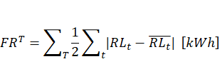
(24)
where FR: Flexibility requirements, T: Time period, t: time step, RLt: Residual Load over all t within T; ![]() : average Residual Load over all t within T.
: average Residual Load over all t within T.
2. Contribution of energy storage to the flexibility requirements (FRT,es) sub-metric evaluation: different technologies, such as dispatchable units, storage systems, interconnectors, and demand-side management technologies, can impact the flexibility requirements differently and have the ability to adjust generation flexibly to match residual demand. In the case of the S.2.2 indicator, the contribution of energy storage is considered. The next generation supplied by the energy storage system is subtracted from the residual load curve. This assessment reveals the difference in flexibility requirements compared to the standard residual load curve, allowing to determine the unique contribution of energy system. This process gives valuable insights into how energy storage systems can effectively address the dynamic flexibility needs of the energy system, considering its contributions to the deviation between actual and normal load curves at each time step. Accordingly, the correlation can be updated to evaluate the effectiveness of the energy storage technologies in meeting the changing demands of the power system, according to Equation (25).
(25)
where ![]() : represents the contribution of the energy storage to the flexibility requirements at a specific timescale T;
: represents the contribution of the energy storage to the flexibility requirements at a specific timescale T; ![]() : the energy supplied by the energy storage at time step t.
: the energy supplied by the energy storage at time step t.
![]() represents the amount of energy storage that can contribute to balancing the grid and meeting the changing demand. If
represents the amount of energy storage that can contribute to balancing the grid and meeting the changing demand. If ![]() is positive, it means that the energy storage helps meet the flexibility requirements by providing additional flexibility. If
is positive, it means that the energy storage helps meet the flexibility requirements by providing additional flexibility. If ![]() is negative, it means that other technologies alone are sufficient to meet the requirements, and energy storage might not be needed to the same extent.
is negative, it means that other technologies alone are sufficient to meet the requirements, and energy storage might not be needed to the same extent.
3. S.2.2 score evaluation: the metric corresponding to the energy storage factor, which is the contribution of the energy storage to the flexibility requirements to the flexibility requirements of the system in case of absence of any energy storage system, is estimated as the ratio of FRT,es (quantified in step 2) to FRT (quantified in step 1), expressed as a apercentage. Subsequently, S.2.2 score is estimated according to Equation (26) as a ratio in which the numerator is the difference of the score of the aforementioned metric against the score of the baseline metric (Tbaseline) for the flexibility requirement, and the denominator is the score of the same baseline metric. The ratio is multiplied by 100, so that the indicator score can be expressed as a dimensionless value that varies between 0 and 100
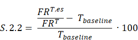
(26)
The indicator quantifies the contribution of energy storage as a solution to reduce the flexibility requirements and thus facilitate the energy system. If the S.2.2 score is negative, an energy storage is not needed. If the S.2.2 score is positive, an energy storage system can reduce the flexibility requirements of the energy system.
The benchmark for comparing the behaviour of different buildings, neighbourhoods, cities, and countriescan be based on the flexibility requirements and energy storage power (Koolen et al., 2023), as summarised in Table 10.
Table 10. Flexibility requirements and energy storage power.
| Flexibility Requirements | ||
| Current 2022 | Future 2050 | |
| European Union | 120 TWh | 2200 TWh |
| Italy | 25 TWh | 160 TWh |
| Energy storage power | ||
| Current 2022 | Future 2050 | |
| European Union | 60 GW | 600 GW |
Source: Koolen et al., 2023.
At neighbourhood/urban scale, multiple building-scale assessments need to be performed by considering each building within the designated area and applying the same three-step framework defined for the evaluation of the S.2.2 score at the single building scale. Subsequetly, the S.2.2 score is estimated as a weighted average of the indicator scores corresponding to the separate building scale assessments.
3.5.4 Example (S.2)
The example for the evaluation of the S.2 KPI is carried out by considering two projects referring to a building and an urban scale project, respectively.
The building scale project is new naturally ventilated multifamily residential building with auseful internal floor area equal to 2700 m3, located in Turin (Italy). The building is equipped with a photovoltaic (PV) system and solar thermal collectors for DHW and space preheating. The PV produces 55110 kWhe/year and exports 23547 kWhe/year to the electric grid, while the solar collectors generate a thermal output of 39375 kWhth/year. The electric energy produced by the PV and not used directly for the building energy uses is first stored in batteries. This considers the time mismatch between production and use of electricity depending on the building load variations. Matching factors of produced and used electricity are according to ISO 52000-1 (ISO, 2017a). If the storage is fully charged, the electric energy is exported. In addition, the building imports 58360 kWhe/year from the electric grid and is equipped with a natural gas boiler with an annual natural gas consumption of 6422 m³ that is only used for space heating and supplementary for DHW, for periods not covered by solar thermal.
The evaluation of the S.2 KPI to maximise the use of sustainable energy in the built environment (S.2) depends on the scores of S.2.1and S.2.2 indicators.
The S.2.1 score is evaluated according to the four-step framework (Section 3.5.2) to estimate the scores of specific sub-metrics and metrics to finally evaluate the indicator score, as follows:
- Annual delivered energy demand (EP) sub-metric evaluation: The annual total delivered electricity for building operations (Ec) is the balance of the total annual electricity produced by all on-site plants (Ep) like from photovoltaics, the electric energy produced by all local plants that is exported (Ee), as it is not used by the building, and the imported electricity (Ei) from the grid:
The onsite solar thermal energy is used for building DHW and space preheating (Qp) and the exported energy (Qe) is zero. The imported thermal energy (Qi) is estimated as the product of the natural gas consumption with the lower heating value:
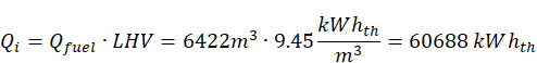
In this example, the natural gas is only used for the specific building services. The annual total delivered thermal energy demand (Qc) for building operations for all forms of energy, i.e. renewables and natural gas becomes:
- Annual total delivered energy demand for building operations covered by renewable energy sources (ERES) metric evaluation: Considering the onsite renewable energy generation for electricity, the total annual delivered demand for building operations covered by renewables is the balance of the total annual electricity produced by all on-site plants (Ep), the exported electricity (Ee) not used by the building, and the imported electricity from renewable sources delivered by distant/nearby generators that is zero in this example:
The onsite renewable energy generation for thermal energy includes the onsite thermal energy production from the solar collectors and used for building operations (i.e. DHW and space preheating), the exported energy that is zero and the imported thermal energy from renewable sources delivered by distant/nearby generators that is also zero in this example:
- Renewable energy (REStot) metric evaluation: the share of the renewable energy (estimated in step 2) relative to the annual total delivered energy demand for building operations (evaluated in step 1) is estimated by using Equation (22). Specifically, the share of renewable energy relative to the total delivered electricity and thermal energy is evaluated separately, according to Equation (27) and (28), respectively.
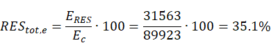
(27)
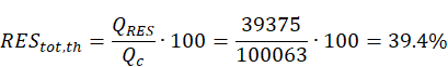
(28)
The total share of renewable energy relative to the annual total delivered energy demand, including both electricity and thermal energy, for building operations is estimated by using Equation (22), as follows (Equation (29)):
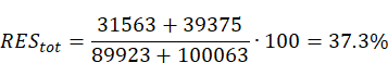
(29)
S.2.1 score evaluation: having estimated the (REStot) metric, S.2.1 score is evaluated in relation to the EU context, considering the score of the baseline metric for the average use of renewable in EU buildings equal to 23.5 % (SWD, 2021). Depending on available local or national data, it may be more appropriate to use different scores of the baseline metric for thermal and electrical energy. The S.2.1 score, considering togheter the use of renewables for electrical and thermal energy, is obtained by using Equation (23), as follows (Equation (30)):

(30)
The S.2.1 score indicates that building scale project analysed accounts for an integration of the use of renewables exceeding the baseline metric of 58.7 %. However, further steps to improve the indicator performance relate to the replacement of gas-fired boiler with a heat pump, the use of solar thermal collectors and the heat-pump as a backup for DHW, and the use of green electricity from the main power supply to enhance the building environmental performance and minimise its carbon footprint.
The S.2.2 score is evaluated according to the four-step framework (Section 3.5.3) to estimate the scores of specific sub-metrics and metrics to finally evaluate the indicator score, as follows:
- Flexibility requirements over the time period (FRT) sub-metric evaluation: the hourly energy profile of the PV performance during a typical spring day and the corresponding residual load and average residual load profiles are illustrated in Figure 20.
Figure 20. Example (S.2): hourly PV energy performance and residual load profile
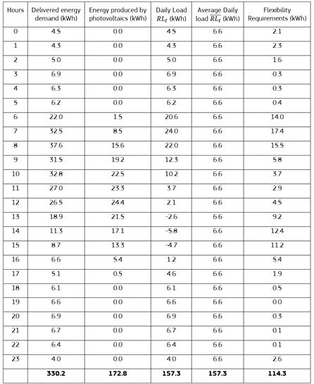
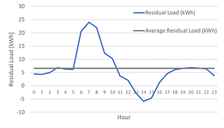
Source: JRC
Having estimated the residual load and the average residual load, the daily FRT sub-metric is evaluated by using Equation (24), as follows (Equation (31)).
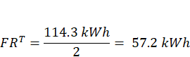 |
(31)
2. Contribution of energy storage to the flexibility requirements: the impact of an energy storage system on hourly energy withdrawals from the grid is illustrates in Figure 21. It demonstrates that the withdrawal pattern deviates less from the daily average trend when energy storage is used, compared to the case without it.
Figure 21. Residual load profile with energy storage system
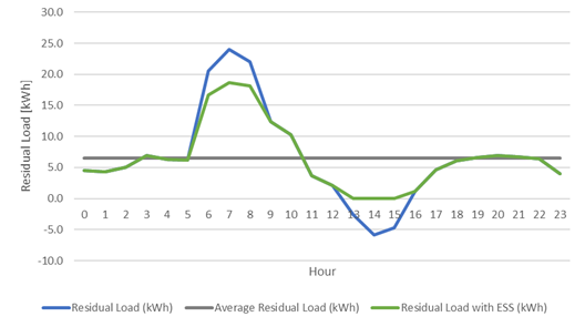
Source: JRC
This represents the energy supplied by the ESS for one day. The influence of the energy storage system in respect to the system without energy storage can be calculated as the percentage of decreasing in the energy flexibility requirements.
3. S.2.2 score evaluation: The baseline for the energy storage factor is taken as 15 %. Depending on available local or national data, it may be more appropriate to use different baselines. The value of the relative indicator then becomes:
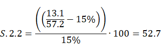
Discussion:
- The contribution of the energy storage is positive, indicating that the energy storage system is reducing by 22.9% the flexibility requirements of the system.
- Energy storage balances energy supply and demand, facilitating the total delivered energy demand (S1.1). The energy consumption patterns, can be used to identify when excess energy should be stored during periods of low consumption and when stored energy should be discharged during peak demand. In essence, the relationship between energy storage and energy consumption is driven by the need to efficiently manage and optimize energy use, making it a key factor in sizing and implementing effective energy storage solutions.
- Energy storage systems are closely intertwined with renewable energy sources due to their ability to tackle the intermittent nature of renewables. These systems enable the storage of excess energy generated by renewables during favourable conditions and make it available when needed, ensuring a consistent and reliable energy supply. Energy storage plays a critical role by mitigating intermittency, optimizing renewable energy utilization, and enhancing grid stability.
- Energy peak demand (S1.2) refers to the periods when energy demand reaches its highest levels, often due to factors like extreme weather, increased industrial activity, or high usage periods. During such peaks, the strain on the electrical grid can be immense, potentially leading to brownouts or blackouts. This is where energy storage systems come into play. Energy storage solutions store excess energy during low-demand periods and release it during peak demand. This not only enhances grid reliability but also allows for the efficient utilization of renewable energy sources, which may generate surplus energy at times when demand is low.
- Energy storage may also be critical if different energy tariffs are used to mitigate the use of energy from the grid at periods with lower tariffs.
Having evaluated the scores of S.2.1 and S.2.2 indicators, S.2 score is estimated by using Equation (20) and considering the indicator weights corresponding to the combination of the project classification according to scale, type, and main use into building, newbuild, and residential, respectively (Table 5). Hence, S.2 results into a score estimated equal to 54.8 that corresponds to the Good performance class (Figure 17, newbuild/residential), as reported in Table 11.
Table 11. Example of S.2 evaluation (building scale).
| Indicator | S.2.1 | S.2.2 |
| Indicator score | 58.7 | 52.7 |
| S.2 score | 0.35 • 58.7 + 0.65 • 52.7 = 54.8 | |
| S.2 performance class | Good | |
| S.2 performance class score (PCSS.2) | 70 | |
Source: JRC
In the building decarbonisation era, eliminating the use of natural gas and on-site combustion, with heat pumps using green electricity would result to even higher performance of S.2 indicator along with S.1 and S.3, among others.
At neighbourhood/urban scale, the objectives are similar to maximise the use of sustainable energy in the area by utilising renewables and energy storage at a larger scale, taking advantage of synergies among buildings. The use of sustainable energy in the area combines the same two indicators, using the corresponding weights for new and renovated buildings, and for different building types. The assessment for the share of renewables in the entire area that beyond residential it includes non-residential buildings may be more challenging. In this case, the installation of systems that exploit renewables may not be possible to be integrated on the buildings. The approach will then be best served with nearby and distant energy generators inside the area’s boundaries. For the energy storage, all residential buildings have solar thermal collectors to cover the DHW demand, coupled with high performance heat pumps for preheating, PVs for on-site, nearby and distant electricity generation, minimising transmission and distribution losses, with the appropriate energy storage and necessary controls to balance peak loads and demand.
— Assess S.2 – Maximise the Use of Sustainable Energy
For a new neighbourhood with residential and non-residential buildings, the residential use is considered as this results into the main use in the neighbourhood. The two indicators are assessed for all buildings and the corresponding scores of the indicators are 83 for S.2.1 and 68 for S.2.2. The S.2 score is evaluated by using Equation (21), considering the indicator weights related to the combination of the project classification as new/residential (Table 5). S.2 results into a score equal to 77.7 that corresponds to the Excellent performance class (Figure 18, new/residential), as reported in Table 12.
Table 12. Example of S.2 evaluation (neighbourhood/urban scale)
| Indicator | S.2.1 | S.2.2 |
| Indicator score | 83 | 68 |
| S.2 score | 0.65 • 83 + 0.35 • 68 = 77.7 | |
| S.2 performance class | Excellent | |
| S.2 performance class score (PCSS.2) | 100 | |
Source: JRC.
3.6 Minimise greenhouse gas emissions from the built environment (S.3)
3.6.1 Description and assessment
At building scale, minimise greenhouse gas emissions from the built environment (S.3) KPI assesses the Global Warming Potential (GWP) intended as the total amount of GHG emissions associated with the construction, operation, and demolition of a building during its entire lifecycle. This is closely related to a life cycle assessment (LCA), which is used to evaluate the environmental impacts of products, processes, or systems from cradle to grave, according to ISO 14040-44 (ISO, 2006). S.3 is evaluated through the following two indicators:
— Operational greenhouse gas (GHG) emissions (S.3.1).
— Embodied greenhouse gas (GHG) emissions (S.3.2).
S.3 score is evaluated according to Equation (32) using different indicator weights (wS.3.j) depending on the different combinations of the project classification according to type (i.e. newbuild or renovation)/main use (i.e. residential or non-residential) of a building scale project, as reported in Table 5. As example, the indicator weights within Equation (32) correspond to the combination of the project classification according to scale, type, and use into building, renovation, and residential, respectively.
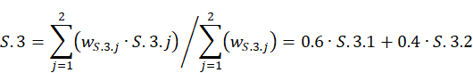
(32)
The S.3 KPI thresholds to associate the KPI score to the corresponding KPI performance class, at building scale, are illustrated in Figure 22.
Figure 22. S.3 performance classes and thresholds (building scale).

Source: JRC
At neighbourhood/urbanscale, minimise greenhouse gas emissions from the built environment (S.3) KPI is assessed through the following two indicators:
— Operational greenhouse gas (GHG) emissions (S.3.1) from all buildings within aneighbourhood/urban scale project.
— Carbon sequestration (S.3.2) that occurs in above-ground growing biomass, such as forestry and in below-ground soil.
S.3 score is evaluated according to Equation (33) by using different indicator weights (wS.3.j) depending on the different combinations of the project classification according to type (i.e. newbuild or renovation)/main use (i.e. residential or residential/non-residential) of a neighbourhood/urban scale project, as reported in Table 5. As example, the indicator weights within Equation (33) refer to a project classified as neighbourhood scale, renovation type, and residential main use.
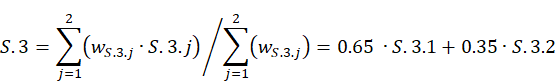
(33)
The S.3 KPI thresholds to associate the KPI score to the KPI performance class, at the neighbourhood/urban scale are illustrated in Figure 23.
Figure 23. S.3 performance classes and thresholds (neighbourhood/urban scale).

Source: JRC.
3.6.2 Operational greenhouse gas (GHG) emissions (S.3.1)
At building scale, the operational greenhouse gas (GHG) emissions (S.3.1) indicator is assessed based on Level(s) indicator 1.2 ‘Life cycle global warming potential’ (Dodd et al., 2021) that addresses emissions from all phases of the lifecycle of a building, encompassing both operational and embodied emissions, according to the European standards EN 15978 (CEN, 2011) and EN 15804 (CEN, 2012d).
The S.3.1 indicator is evaluated focusing on the use phase of the building life cycle, which corresponds to the module B6 “Operational Energy use” of the standardised life cycle phases of a building, according to EN 15978 (CEN, 2011). Non-energy-related systems that contribute to GHG emissions, such as the provision of potable water, wastewater treatment or refrigerants leakage, are excluded from the scope. S.3.1 assesses the reduction of the annual operational GHG emissions of a building scale project, against a baseline score, corresponding to the average annual operational GHG emissions of the EU and/or national reference building stock, to evaluate the progress towards the performance of zero-emissions building.
The S.3.1 score, which ranges between 0 and 100, is evaluted according to a three-step framework that consecutively estimate the score of specific sub-metrics and metrics to finally evaluate the indicator score, as follows:
- Annual delivered energy sub-metric evaluation: the delivered energy to be estimated (also refer to the S.1.1 evaluation in Section 3.4.2) is intended as the energy, expressed per energy carrier (Q), supplied to the technical building systems, to satisfy the building uses taken into account. The energy is delivered to the building in the form of electricity, heat and fuel in order to satisfy the building services, according to ISO 52000-1 (ISO, 2017a). Additional building services can be integrated depending on the use of the building (e.g. hospitals, retail, etc.) and quantified separately.
- Annual operational GHG emissions (annual OGHG) metric evaluation: The annual OGHG metric is estimated by summing the products of the annual delivered energy per energy carrier (Q), estimated in step 1, by the corresponding GHG emission factors (kem), and normalising the obtained sum per unit useful internal floor area (Au), according to Equation (34). The GHG emissions factors are collected from national or transnational databases.
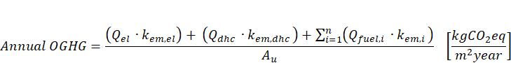 |
(34)
The variables in Equation (34) are defined, as follows:
a) Qfuel,i is the total annual delivered energy from the i-th fuel (kWhth) used for the building specific technical building systems (thermal energy of fossil fuels is estimated by multiplying the quantity of fuel by the lower heating value of the fuel, e.g. m3 of natural gas is multiplied by 9.45 kWhth/m3).
b) kem,i is the GHG emissions factor of the i-th fuel (kgCO2-eq/kWhth),
c) Qel is the total quantity of annual electrical energy from the grid (kWhe),
d) kemis the GHG emissions factor of the electrical energy from the grid (kgCO2-eq./kWhe),
e) Qdhc is the total quantity of annual energy from district heating/cooling (kWhth),
f) kem,dhc is the GHG emissions factor of energy from district heating/cooling (kgCO2-eq/kWhth),
The following values of GHG emission factors for different energy carriers (expressed in kgCO2-eq/kWh) can be considered (Lo Vullo et al., 2022): 0.202 (for natural gas), 0.268 (for oil), 0.007 (solid biomass), 0.356 (coal), 0 (from renewables), and for average EU electricity at 0.254 kgCO2-eq/kWh for 2020. Due to the high annual variability, the most recent emissions factors for electricity in EU-27 should be used for future calculations (EEA Greenhouse gas emission intensity n.d.).
3. S.3.1 score evaluation: the S.3.1 score is assessed according to Equation (35) as a ratio, in which the numerator is the difference of the scores of a baseline metric (Tbaseline) and the annual OGHG metric (evaluated in step 2) and the denominator is the score of the same baselinemetric, multiplied by 100, so that the indicator score can be expressed as a dimensionless value that varies between 0 and 100. The score of the baseline metric (Tbaseline) corresponds to the average annual operational GHG emissions per unit floor area (expressed in kgCO2-eq/m2year) of the national or EU building stock to which the building scale project belongs, according to building type and climatic zone.
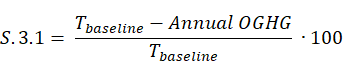 |
(35)
If the annual OGHG metric score is lower than the Tbaselinemetric score, S.3.1 results into a positive score. The higher the indicator score, the better the building performance related to the reduction of the operational GHG emissions, noting though that the indicator maximum score is 100. If the annual OGHG metric score is greater than the baseline metric score, leading the difference in the numerator to be negative, S.3.1 results into a negative score indicating that the building performance does not satisfy the baseline metric, providing an increase of the annual operational GHG emissions compared to the baseline metric, thus the indicator score is assumed equal to zero (0). Specifically, a building scale project with zero annual operational GHG emissions will obtain a S.3.1 score equal to 100, indicating a top performance (i.e. zero-emissions) building, whereas a baseline performance building will reach a S.3.1 score equal to 0. Buildings should at least meet the minimum requirements for GHG emissions. Based on the S.3.1 score, different scenarios to evaluate possible design improvements of a building scale project can be defined to obtain more effective reduction of operational GHG emissions.
The score of the baseline metric to be used in Equation (35) is determined as an average of the annual operational GHG emissions per unit floor area of the building stock, at national or EU level, to which the building belongs, according to Equation (36). The score of the baseline metric shall be specific per building use (e.g. residential, office, retail, etc.) and climate zone in which the building is located. In case of mixed-use buildings, the baseline metric score shall be estimated as the weighted average of the baseline annual operational GHG emissions of each occupancy considering their indoor useful area. In equation (35), Tbaseline,i is the baseline annual operational GHG emissions of the i-th occupancy (kgCO2-eq/m2.year) and Ai is the internal useful floor area of the i-th occupancy (m2).
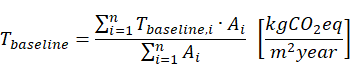
(36)
The score of the baseline metric varies depending on the building stock considered at national or EU level, thus corresponding to the average annual operational GHG emissions of the national or EU building stock, respectively. Ifrelevant data, at national and/or EU level, per building type or climate zone are not available, it is possible to use more generic and approximate data, reporting its source. The use of more accurate input data for the annual operational GHG emissions per building type and climate zone, will lead to a more accuratescore of the indicator.
At EU level, representative scores of a baseline metric are summarised in Table 13. These scores are expressed as annual operational GHG emissions per unit floor area of building differentiated by high-rise, multi-family, and single-family building for three climate zones (Z) representative of South, Central, and North Europe, identified by specific HDD-ranges.
Table 13. Representative annual operational GHG emissions of buildings by climatic zone in Europe
| Climatic Zone | High rise buildings (kgCO2 eq / m2.y) | Multi-family buildings (kgCO2 eq / m2.y) | Singlefamily houses (kgCO2 eq / m2.y) |
Z1: South Europe (564 to 2500 HDD) | 18 | 30 | 65 |
Z2 Central Europe (2501 to 4000 HDD) | 40 | 55 | 85 |
Z3: North Europe (4000 to 5823 HDD) | 55 | 90 | 115 |
Source: data from Gervasio and Dimova, 2018.
Furthermore, at EU level, it is possible to analyse the S.3.1 score in relation to the EU 2030 binding target, aimed at reducing the GHG emission by at least 55 %, compared to 1990 levels, towards the climate-neutrality by 2050, according to the European climate law (Regulation, 2021/1119)., Hence, a score of S.3.1, estimated by using the score of the baseline metric at EU level, being greater than 55 is considered as positive in relation to the EU 2030 target of GHG emission reduction.
At neighbourhood/urban scale, the operational GHG emissions assessment of a single building can be scaled up to assess the reduction of GHG emissions at a larger scale.Specifically, multiple building-scale assessments need to be performed by considering each building within the area of the neighbourhood/urban scale project and applying the same three-step framework defined for the evaluation of the S.3.1 score at single building scale to assess the annual operational GHG emissions of each building within the designated area. Subsequently, the S.3.1 score at neighbourhood and urban scale is estimated as the sum of the annual OGHG metric scores corresponding to the separate building scale assessments, normalised per inhabitant, according to ISO 37120 (ISO, 2018) and relevant guidelines for reporting climate and energy (Covenant of Mayors, 2020). Hence, the S.3.1 score at neighbourhood/urban scale is expressed in tonnes CO2-eq/inhabitant. Data on the number of inhabitants within the area of the neighbourhood/urban scale project can be collected from the statistical offices of municipalities. The score in tonnes CO2-eq/inhabitant is then compared to a baseline value, similar to the procedure for the building scale. To help define the baseline value, the first total value of annual operational GHG emissions can be used as a baseline year to set emission reduction targets (e.g., 2030, 2050) and to monitor progress over time.
3.6.3 Embodied GHG emissions (building scale) or carbon sequestration (urban scale) (S.3.2)
At building scale, the embodied GHG emissions (S.3.2) relies on the assessment of the overall Global Warming Potential (GWP) due to the emitted GHGs over a reference study period, generally corresponding to the service life of a common building (i.e. 50 years). The system boundary to carry out the analysis for the evaluation of S.3.2 indicator is “from cradle to grave”, thus focusing on different stages of the lifecycle of a building scale project, including the production stage, the construction process, the use stage, and the end of life, corresponding to specific ‘modules’ of the standardised building lifecycle (Figure 24), according to EN 15978 (CEN, 2011) and elaborated by Levels(s) indicator 1.2 (Dodd et al., 2020b). Specifically, the embodied GHG emissions in buildings are generated at the product and construction stage (i.e. modules A1-5), the use stage (i.e modules B1-5) and the end-of-life stage (i.e. modules C1-4). In the case of a new building scale project, the analysis to estimate the embodied GHG emissions focuses on A1-A5, B1, B4, B5, and C1-C4 modules, whereas B2 and B3 modules that refer to GHG emissions from the maintenance and repair of a building are not included in the system boundary due to issues related to data availability and data precision, also considering that these stages have a low carbon impact compared to other lifecycle stages. In the case of a renovation building scale project, the system boundary shall encompass all modules that relate to the extension of the building service life, namelyfrom B1 module onwards, as the stages relating to the original production (A1-3) and construction (A4-5) have already taken place. Hence, the GHG emissions associated with materials used in the construction process for the renovation shall be allocated to the use stage (B). Module D that concerns the benefits and loads arising from the reuse of products or the recycling or recovery of materials and compoenets is optional. If module D is included in the system boundary, the results shall be reported separately. In case of demolition of existing buildings on the site prior to the construction of a new building, the benefits and loads arising from the recovery of demolition shall be considered to be outside of the system boundary. The benefits and loads must therefore be eventually allocated to the previous building to avoid double counting.
Figure 24. Standardised life cycle stages (i.e. modules) of a building according to EN 15978,
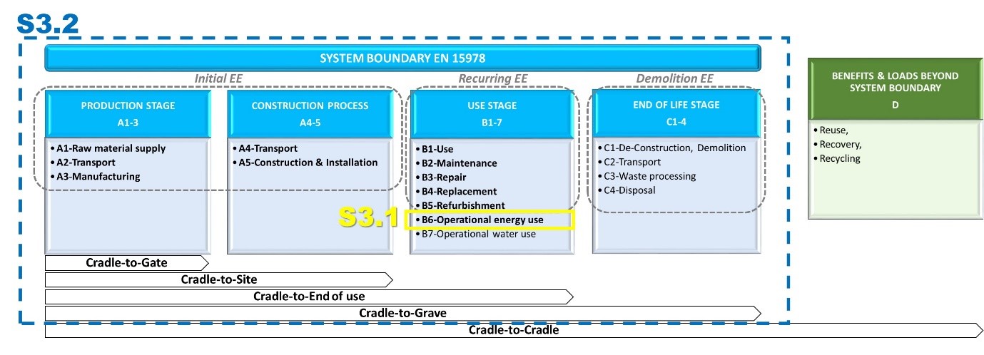
Source: Adapted from CEN, 2011.
The largest contribution of embodied GHG emissions in European buildings (Figure 25) occurs during the production stage (i.e. modules A1-3), with a mean value of about 300 kg CO2-eq/m2, ranging from 70 to 520 kg CO2-eq/m2 (Röck et al., 2022). The second largest contribution occurs during the use phase (i.e. moduels B1-4), with a mean value of around 120 kgCO2-eq/m2, which represents the total amount of embodied GHG emissions from cleaning, maintenance, and replacement activities taking place over a 50-year reference study period (Röck et al., 2022).
Figure 25. Embodied GHG emissions per unit floor area for different life cycle stages
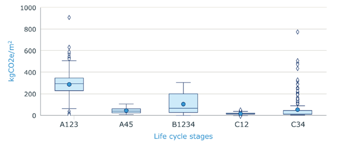
Source: Röck et al., 2022.
The S.3.2 indicator assesses the reduction of the embodied GHG emissions of a building scale project in reference to a baseline score, corresponding to the average embodied GHG emissions of the national and/or EU building stock. The assessment of the GHG embodied emissions of a building is a complex process, which shall be performed through the LCA methodology, according to ISO 14040-44 (ISO, 2006a, b), by using a robust LCA software tool in compliance with the European standard EN 15978 (CEN, 2011). The assessment requires comprehensive data on construction products and environmental impacts over the entire lifecycle of the building.
The S.3.2 score, which ranges between 0 and 100, is evaluted according to a four-step framework that consecutively estimate the score of specific sub-metrics and metrics to finally evaluate the indicator score, as follows:
- Bill of Quantities (inventory) preparation: the inventory of all construction products integrated in the building scale project, in the form of a Bill of Quantities (BoQ) needs to be prepared. The construction products and materials to be included in the inventory refer to building elements, components, technical installations, external works, etc., classified through different tiers, according to Level(s) indicator 2.1 (Donatello et al., 2021a), as listed in Table 14. In case of a renovation building scale project, only the new construction products added to the building shall be taken into consideration, thus excluding the existing ones. The inventory accounts for the bill of quantities of all construction products, used in a newbuild orrenovation building scale project, that are included in the physical scope of the assessment. The system boundaries include the A1-A5, B1, B4, B5, and C1-C4 modules for a newbuild building scale project; whereas the the B1, B4, B5, B6, C1-C4 moduels are considered for a renovation building scale project.
Table 14. Classification of building elements and components for the bill of quantities preparation.
| Tier 1 | Shell (substructure and superstructure) | ||
| Tier 2 | Foundations (substructure) | Tier 3 | Piles, Basement, Retaining walls |
| Load bearing structural frame | Frame (beams, columns and slabs), Upper floors, External walls, Balconies | ||
| Non-load bearing elements | Ground floor slab, Internal walls, partitions and doors, Stairs and ramps | ||
| Façades | External wall systems, cladding and shading devices, Façade openings (including windows and external doors), External paints, coatings and renders | ||
| Roof | Structure, Weatherproofing | ||
| Parking facilities | Above ground and underground (within the curtilage of the building and servicing the building occupiers) | ||
| Tier 1 | Core (fittings, furnishings and services) | ||
| Tier 2 | Fittings and furnishings | Tier 3 | Sanitary fittings, Cupboards, wardrobes and worktops (where provided in residential property), Ceilings, Wall and ceiling finishes, Floor coverings and finishes |
| In-built lighting system | Light fittings, Control systems and sensors | ||
| Energy system | Heating plant and distribution, Cooling plant and distribution, Electricity generation and distribution | ||
| Ventilation system | Air handling units, Ductwork and distribution | ||
| Sanitary systems | Cold water distribution, Hot water distribution, Water treatment systems, Drainage system | ||
| Other systems | Lifts and escalators, Firefighting installations, Communication and security installations, Telecoms and data installations | ||
| Tier 1 | External works | ||
| Tier 2 | Utilities | Tier 3 | Connections and diversions, Substations and equipment |
| Landscaping | Paving and other hard surfacing, Fencing, railings and walls, Drainage systems | ||
Source: Adapted from Donatello et al, 2021b.
- GWP of construction products (GWP‑total) sub-metric evaluation: data concerning the environmental impacts in terms of total Global Warming Potential of all the construction products included in the inventory defined in step 1 need to be collected for the life cycle stages included in the system boundary of the assessment. Relevant data on the GWP of construction products is available from the Environmental Product Declarations (EPDs) or in LCA databases. Depending on the type of construction product, the GWP-total values may be normalised per functional unit of the product, e.g. mass (kgCO2-eq/kg), volume (kgCO2-eq/m3), area (kgCO2-eq/m2), etc.
- The data concerning the GWP-total of construction products must be contextualised to the region where the building is located. In general, the GWP depends on the national energy mix that varies from country to country (e.g. different share of renewable energy, use of nuclear energy). For example, if the assessment is performed in Italy (with a national energy mix that is dominated by fossil fuels (79 %), no nuclear energy used) it would not be appropriate to use a French LCA database (national energy mix with a prevalence (42 %) of nuclear energy). Other influencing factors that must be contextualised include the transport mode of materials (e.g. local, national, origin of imported materials).
Accordingly, the degree of confidence in the results depends upon the quality of the data used. The following data hierarchy shall be used to prioritise data resources: (i) use of data from EPDs specific for the construction products used in the building; (ii) use of average data from EPDs describing average products and estimated using representative average data; (iii) use of average data from LCA databases that are compliant with the EN 15804 (CEN, 2012). If the environmental data are from other sources which are not in compliance with EN 15804 (CEN, 2012), the following minimum data quality requirements apply: (i) data shall have been checked for plausibility and compliance with the rules of EN 15804 (CEN, 2012); (ii) data should be as current as possible with the last update not being older than 10 years for generic data and 5 years for manufacturer’s data; (iii) datasets for estimations should be based on one-year averaged data, if relevant, and reasons for a different assessment period shall be listed; (iv) the technological processes associated with the product shall be representative of the declared product or product group; and (v) the technological processes shall be representative of the region where the production is located.
- Embodied GHG emissions of building (EGHGb) metric evaluation: the embodied GHG emissions metric is estimated as the amount of embodied GHG emissions of the entire building scale project (i.e. GWP‑totalb) normalised per its internal useful floor area (Au), according to Equation (37).
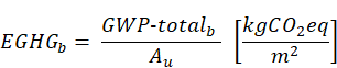
(37)
The embodied GHG emission of the building are estimated on the basis of the quantities of building products estimated in step 1 and the GWP-total values collected in step 2, according to the rationale provided in
Figure 26. The assessment shall be carried out for a reference study period of 50 years, corresponding to the service life of a common building. However, the reference study period may differ from the required service life of the building.
Figure 26. Evaluation of embodied GHG emissions of each construction product in a building scale project.
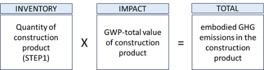
Source: JRC.
The lifespan of building parts and elements, whichis used to derive the times of replacement during the reference study period of 50 years, can be estimated in various ways: (i) according to the factor methodology in ISO 15686-8 (ISO, 2008), (ii) using data provided by manufacturers and suppliers, or (iii) using generic lifespans from LCA tools, building costing tools or other guidance for typical service lives listed in Level(s) indicator 2.1 ‘Bill of Quantities, materials and lifespans’ (Donatello et al., 2021b, Dodd et al. 2021a).
S.3.2 score evaluation: the S.3.2 score is estimated according to Equation (38) as a ratio, in which the numerator is the difference of the score of a baseline metric (Tbaseline) of embodied GHG emissions (expressed in kg CO2-eq/m2) and the score of the EGHGbmetric (evaluated in step 3) and the denominator is the score of the same baseline metric (Tbaseline), multiplied by 100, so that the indicator score can be expressed as a dimensionless value that varies between 0 and 100.
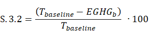
(38)
If the EGHG metric score is lower than the Tbaselinemetric score, S.3.2 results into a positive score. The higher the indicator score, the better the building performance related to the reduction of embodied GHG emissions, noting though that the indicator maximum score is 100. If the EGHG metric score is greater than the baseline metric score, leading the difference in the numerator to be negative, S.3.2 result into a negative score indicating that the performance does not satisfy the baseline metric, thus the indicator score is set to zero (0). Buildings should at least meet the minimum requirements for GHG emissions. The EGHG metric is compared with the baseline metric scoreto evaluate the building performance related to its embodied GHG emissions. A very high performance building will have an S.3.2 score greater than 50, which implies a building with embodied GHG emissions that are less than half of the average embodied GHG emissions of the baseline EU or national building stock. Based on the S.3.2 score, different scenarios to evaluate possible design improvements of a building scale project can be defined to obtain more effective reduction of embodied GHG emissions.
The score of the baseline metric to be used in Equation (38) corresponds to an average of embodied GHG emissions per unit floor area of the national or EU building stock to which the building scale project belongs, according to building type (i.e. newbuild/renovation), main construction material, and use. Relevant studies in this direction provides data useful to set the score of a baseline metric of embodied GHG emissions per unit floor area for newbuild (Röck et al., 2022) and renovation (Brown et al., 2024) projects, as follows:
- Newbuild project — Based on data from LCA studies in 769 buildings in Belgium, Denmark, Finland, France and the Netherlands (Figure 27), the following averages of embodied GHG emissions per unit floor area are estimated for different building use and main construction material, for a reference study of 50 years: (i) residential buildings (550 kgCO2-eq/m2), non-Residential buildings (450 kgCO2-eq/m2), massive concrete buildings (750 kgCO2-eq/m2), massive brick buildings (700 kgCO2-eq/m2), massive timber buildings (500 kgCO2-eq/m2), and for all technical services (e.g., heating, cooling, domestic hot water and sewage systems): 190 kgCO2-eq/m2 (Röck et al., 2022).
Figure 27. Harmonised full life cycle embodied GHG emissions per unit floor area for different building uses
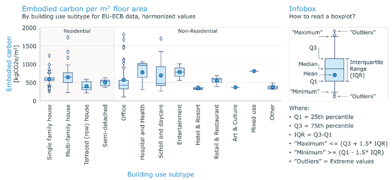
Source: Rock et al., 2022.
- Renovation project — Depending on the nature and depth of the renovation works and the materials used, the increase of embodied GHG emissions is typically less than 50 % of the embodied emissions for a new building (i.e. less than 125–200 kgCO2eq/m2). This figure may be much lower if the renovation aims to improved thermal insulation and heating or cooling systems, without major structural changes (Brown et al., 2014).
The indicator score can provide useful insights to develop life cycle scenarios that can support decision making processes during the design phase of carbon neutral buildings. Specifically, the indicator can be used to evaluate alternative scenarios to:
- Re-use materials/components of an existing building and its structure compared to its demolition and construction of a new building. This is a relevant scenario as the focus shifts from the performance of new buildings to large scale, deep renovation, according to the EU Renovation Wave (COM 2020/662).
- Define the best design strategy (e.g. building structure) to minimise the embodied GHG emissions of the building and meet carbon neutrality requirements. There are various solutions for reducing embodied GHG emissions in buildings, including synergies among various strategies on each of the three pillars of the SER (Sufficiency, Efficiency, Renewables) Framework (Cabeza et al., 2022). The following solutions and strategies can be considered: (i) implement material-efficiency when designing structural systems, (ii) use low-carbon building materials including bio-based materials (e.g. timber) and energy systems, (iii) consider occupational density and sufficiency principles in building design to reduce the building floor area and hence material consumption.
At neighbourhood/urban scale, the carbon sequestration (S.3.2) indicator focuses on carbon captured and stored in ecosystems on land and estimates the carbon stock of ecosystems on land, and the carbon sequestration rate of the ecosystems on land. The indicator is also useful to understand the extent of ecosystems on land in neighbourhood or urban scale projects contributing to the mitigation of GHG emissions, and evaluate the impact of changes in land uses. Captured and stored carbon is referred to as a “carbon pool” that includes living biomass (above and belowground) and soils (IPCC, 2019). The carbon stock is the quantity of carbon contained in a “pool”, meaning a reservoir or system which has the capacity to accumulate or release carbon. The impact of changes in the carbon stock on GHG mitigation for climate protection is often referred to as carbon sink, although it could also act as a net source of emissions.
The S.3.2 score is evaluated accoridng to a three-step framework that consecutively estimates the scores of specific sub-metrics and metrics, to finally evaluate the indicator score, as follows:
- Inventory of ecosystems on land and area evaluation: an inventory of the different ecosystems on land types (e.g. grasslands, shrubs, sparsely vegetated, croplands, forests, wetlands) needs to prepared by quantifying the area of each i-th ecosystem on land type (i.e. Areai, expressed in hectares)
Carbon stock (CS) evaluation: carbon stock shall be estimated as the sum of products of the extension of the i-th ecosystems on land (i.e. Areai, expressed in ha) by the CO2 stock ratio of the i-th ecosystems on land (CSRi, expressed in tCO2), according to Equation (39). Representative values of CO2 stock ratio per the i-th ecosystem on land are reported in Table 15.
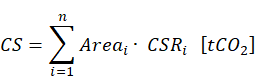
(39)
Table 15. Representative CO2 stock ratios of various land ecosystems.
| Ecosystem | CO2 stock ratio (t CO2/ ha) |
| Cropland | 363 |
| Forest | 424 |
| Grassland | 18 |
| Shrub | 44 |
| Sparsely vegetated | 88 |
| Wetland | 907 |
Source: Hendriks et al., 2022.
Annual carbon sequestration (CSEQ) in ecosystems evaluation: the annual carbon sequestration is estimated as the sum of products of extension of the i-th ecosystem on land (i.e. Areai, expressed in ha) by their annual CO2 sequestration rates (i.e. CSRai, expressed in tonne CO2/ha year), according to Equation (40). Representative values of annual CO2 sequestration ratio per the i-th ecosystem on land are reported in Table 16.
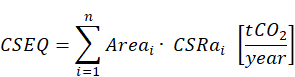
(40)
Table 16. Representative annual CO2 sequestration rates of various land ecosystems.
| Ecosystem | CO2 sequestration rate (t CO2/ha.y) |
| Cropland | 3.3 |
| Forest | 11.0 |
| Grassland | 0.9 |
| Shrub | 0.6 |
| Sparsely vegetated | 0.1 |
| Urban trees | 8.1 |
| Wetland | 0.1 |
Source: Hendriks et al., 2022.
- S.3.2 score evaluation: the metric concerning the annual carbon sequestration is estimated as the ratio of CSEQ (quantified in the step 2) to CS (quantified in the step 2), expressed as a percentage. Subsequently, the S.3.2 score is estimated, according to Equation (41), as a ratio in which the numerator is the difference of the score of the aforementioned metric against the score of the baseline metric (Tbaseline) of the carbon sequestration and the denominator is the score of the same baseline metric, multiplied by 100, so that S.3.2 score can be expressed as a dimensionless value that varies between 0 and 100. A baseline metric of 15 % can be used, which is also considered an overall good visible greenery in urban areas (Tang et al., 2023).
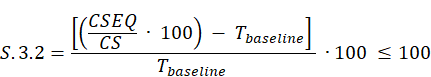
(41)
S.3.2 can also be assessed against a baseline that is set at a value representing the existing status at the beginning of the project. If the metric score is greater than the reference baseline value, S.3.2 score results into is positive value; noting though that the S.3.2 maximum score cannot exceed 100. If the metric score is lower than the reference baseline value leading the difference in the numerator to be negative, S.3.2 score assumes a negative value indicating that the indicator performance does not satisfy the reference baseline, thus S.3.2 score is set equal to zero (0). The score of the baseline metric in Equation Error! Reference source not found. can be set based on the rationale that a neighbourhood/urban scale project should at least meet the local or national minimum requirements for carbon sequestration.
The results are used to assess the share of annual GHG emissions of the city that can be sequestered by ecosystems on land (%). The indicator score provides insights to verify the need to increase the annual carbon sequestration using natural based solutions and evaluate the impact of changes in land use in terms of capacity of carbon sequestration.
3.6.4 Example (S.3)
The example of the S.3 KPI evaluation is carried out by considering a building scale project, which is a new naturally ventilated multifamily residential building with a useful internal floor area of 2700 m2, located in Turin (Italy). Central space heating and domestic hot water (DHW) are served by a natural gas fired non-condensing boiler, whereas cooling is served by local air-to-air heat pumps. The metered annual energy consumption due to natural gas and electricity from the grid is estimated equal to 18 351 m3 and 53 360 kWhe, respectively.
The evaluation of the S.3 KPI to minimise the GHG emissions of the building depends on the scores of S.3.1and S.3.2 indicators.
The S.3.1 score is evaluated according to the four-step framework (Section 3.6.2) to estimate the scores of specific sub-metrics and metrics to finally evaluate the indicator score, as follows:
- Annual delivered energy sub-metric evaluation: following the same analysis as in the example of S.1.1 evaluation, the breakdown of the the delivered energy per energy carrier allocated for the corresponding building services is summarisedin Table 17.
Table 17. Example (S.3): annual delivered energy sub-metric evaluation
| Energy Carrier | kWh/year | Building services | GHG emissions factor (kgCO2-eq/kWh) |
| Natural gas | 173427 | Heating, DHW | 0.21 |
| Electricity | 3202 | Cooling | 0.252 (for 2022 EEA) |
| Electricity | 50158 | Other (e.g. lighting, cooking, white appliances, plug loads) | 0.252 (for 2022 EEA) |
Source: JRC
- Annual operational GHG emissions (Annual OGHG) metric evaluation: based on the annual delivered energy per energy carrier, estimated in step 1, and the corresponding emissions factors for each energy carrier (Table 16),the annual OGHG metric related to heating, DHW, and cooling uses is estimated by using Equation (34), as follows (Equation (42)):
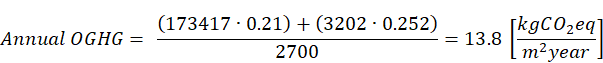
(42)
For sake of completeness, the annual OGHG metric related to all the other uses of the building, e.g. lighting, cooking, etc. (Table 17), is estimated again by using Equation (34), as follows (Equation (43)). Hence, the annual OGHG metric for all uses of the building scale project is equal to 18.5 kgCO2-eq/m2year.
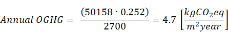
(43)
S.3.1 score evaluation: having estimated the annual OGHG metric, S.3.1 is evaluated in relation to the national, i.e. Italian, and EU context, by setting the scores of the baseline metric at Italian and EU level, as follows:
a) Italian context – S.3.1 is evaluated in relation to the national building stock. Specifically, the building scale project is located in the climate zone E, corresponding to a HDD range equal to 2101–3000, as defined by the Italian decree on thermal energy systems (DPR, 412/1993). The mean value of the operational GHG emissions for buildings located in the Italian climate zone E is 44.7 kgCO2-eq/m2.year (DPR, 412/1993), corresponding to the Tbaseline score at national level. Having estimated the score of the annual OGHG metric for heating, DHW, and cooling uses (Step 2), and the baseline metric score at national level, S.3.1 score is evaluated by using Equation (35), as follows (Equation (44))
(44)
The S.3.1 indicator results into a positive score, pointing out the percentage reduction of the annual operational GHG emissions compared to the average annual GHG emissions of the Italian building stock for climate zone E. If the additional uses of the building scale project, such as cooking, lighting, etc., are considered, the score of the annual OGHG metric for all uses is equal to 18.5 kgCO2eq/m2year (step 2) and the S.3.1 score is found to be equal to 58.6, according to Equation (45).
(45)
b) EU context - S.3.1 is evaluated in relation to the EU building stock. According to data in Table 13, the average value of the annual operational GHG emissions for multi-family buildings located in South Europe is 30 kgCO2-eq/m2.year that is assumed as the Tbaseline score at EU level. Similarly to the Italian context, having estimated the score of the annual OGHG metric for heating, DHW and cooling uses (step 2), and the baseline metric score at EU level, S.3.1 score is evaluated by using Equation (35), as follows (Equation (46)).
(46)
The S.3.1 indicator results into a positive score, indicating the reduction of the annual operational GHG emissions of the buidilng compared to an EU average for South Europe. Similarly, if the additional uses of the building scale project, such as cooking, lighting, etc., are considered, the annual OGHG metric results into a score equal to 18.5 kgCO2eq/m2year (step 2) and the S.3.1 score is found to be equal to 38.3, according to Equation (47).
(47)
The comparison of the S.3.1 scores in relation to the Italian and EU context points out that the building scale project analysed at Italian level exhibits a better performance related to the reduction of operational GHG emissions, mainly depending on the the higher baseline metric score of the national building stock than one of the EU building stock. Furthermore, the comparision of the S.3.1 score at EU level with the EU 2030 target of GHG emission reduction (i.e. 55 %) underlines that the building scale project is on track, if the annual operational GHG emissions related to heating, DHW, and cooling uses are considered, as the indicator score indicates a reduction of the annual operational GHG emissions equal to 54 %. However, considering the total energy consumption and all services, the indicator needs to be improved, as its score indicates a reduction equal to 38.3 %.
The performance of the building scale project can be further impoved by decarbonising the building through the replacement of the on-site combustion of natural gas with a central heat pump using electricity. A zero-emissions building shall not generate any on-site carbon emissions from fossil fuels according to the EPBD recast (Directive 2024/1275). However, the emissions factors for the grid electricity within the budilng scale project analysed are below the EU-27 average. Yet, the GHG emissions will still be lower considering the lower electricity consumption due to a much better energy efficiency performance of a heat pump compared to theboiler currently considered in the project.
The S.3.2 score is evaluated according to the four-step framework (Section 3.6.3) to estimate the scores of specific sub-metrics and metrics to finally evaluate the indicator score, as follows:
- Bill of Quantities (inventory) preparation: relevant data is collected and reported for all building construction products falling into the physical scope of the indicator. Specifically, the bill of quantities of all building elements/components classified by tier 1 in shell, core, and external works, as indicated in Table 14, needs to be prepared. Figure 28 provides an example of the bill of quantities of an external wall system of the building scale project, belonging to the Tier 1 shell. The quantities to be reported in the BoQ are the masses (kg) of materials of the external wallneeded over lifetime.
Figure 28. Example (S.3): bill of quantities of an external wall system
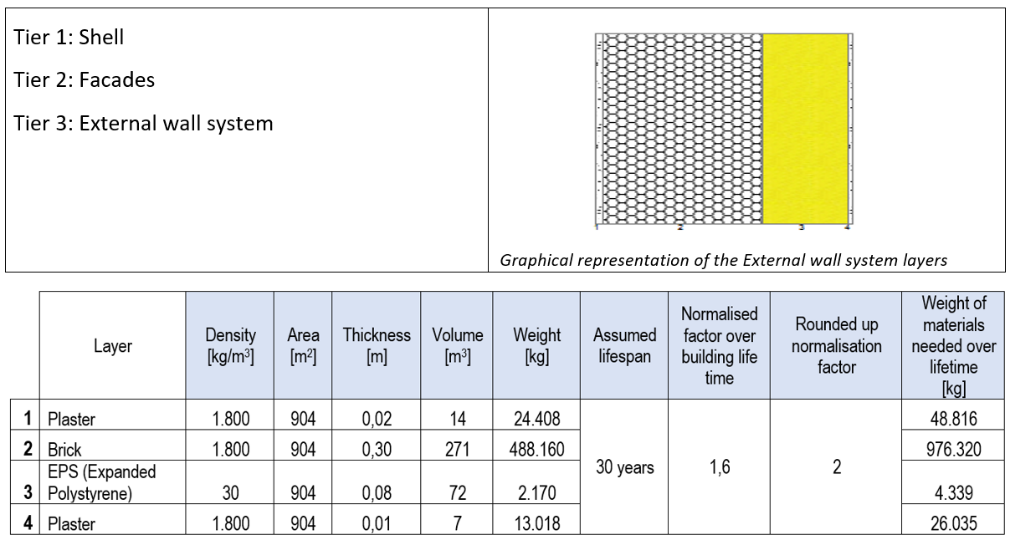
Source: JRC
2. GWP of construction products sub-metric evaluation: The GWP-total valuesper functional unit of mass of product (expressed in kgCO2-eq/kg), are assigned to all the materials in the inventory defined in step 1 by using the available databases, i.e.an Environmental Product Declaration (EPD) for the thermal insulation material and the LCA database for all the other materials composing the external wall, as summarised in Table 18.
Table 18. Example (S.3): GWP-total per functional unit of the construction products of an external wall system
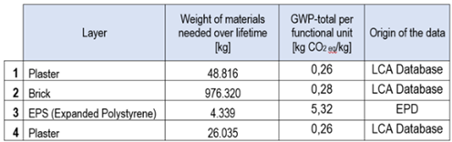
Source: JRC.
- Embodied GHG emissions (EGHG) metric evaluation: based on the BoQ, reported in the step 1, and the GWP-total of each material per functional unit, collected in step 2, the GWP-total for all the building construction materials composing the external wall is estimated according to the rationale in Figure 19. Subsequentlyy, the sum of the GWP-total of each construction products provides the GWP-total of the external wall, as summarised in Table 19.
Table 19. Example (S.3): GWP‑total of an external wall system of the building scale project.
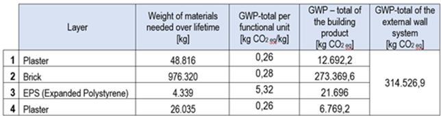
Source: JRC.
The procedure carried out for the external wall system needs to be applied to all the other building elements/components of the building scale project to carry out their GWP-total, grouped by tier 1 in shell, core, and external works, to subsequently summing up these results to obtain the GWP-total of the entire building, as summarised in Table 20.
Table 20. Example (S.3): GWP-total of the building scale project
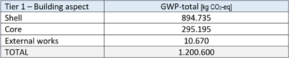
Source: JRC.
Having estimated the GWP-total of the entire building equal to 1200600 kgCO2-eq, considering a reference study period of 50 years, the EGHG metric is estimated by using Equation (37), as follows (Equation (48):
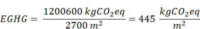
(48)
S.3.2 score evaluation: having estimated the score of the EGHG metric (step 3), and assuming the score for the score of national baseline metric equal to the mean of embodied GHG emissions per unit floor area for new residential buildings (i.e. Tbaseline = 600 kgCO2eq/m2) which is well within the range of the average values for new residential buildings of 400 to 800 kgCO2eq/m2 (Röck et al., 2022), S.3.2 is estimated by using Equation (38), as follows (Equation (49)).
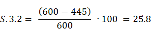
(49)
The indicator results into a positive score equal to 25.8, thus indicating the percentage reduction of the embodied GHG emissions of the building scale project compared to the baseline metric.
Having evaluated the scores of S.3.1 and S.3.2 indicators, S.3 score is evaluated by using Equation (32) and considering the indicator weights corresponding to the combination of the project classification according to scale, type, and main use into building, newbuild, and residential, respectively (Table 5). Hence, S.3 results into a score estimated equal to 43.1 or 37.1, depending on the Italian or EU context, that respectively corresponds to the Good or Acceptable performance class (Figure 22, newbuild/residential), as reported in Table 21.
Table 21. Example of S.3 evaluation (building scale) in relation to the national or EU context.
| Italian context | ||
| Indicator | S.3.1 | S.3.2 |
| Indicator score | 69.1 | 25.8 |
| S.3 score | 0.4 • 69.1+ 0.6 • 25.8 = 43.1 | |
| S.3 performance class | Good | |
| S.3 performance class score (PCSS.3) | 70 | |
| EU context | ||
| Indicator | S.3.1 | S.3.2 |
| Indicator score | 54 | 25.8 |
| S.3 score | 0.4 • 54 + 0.6 • 25.8 = 37.1 | |
| S.3 performance class | Acceptable | |
| S.3 performance class score (PCSS.3) | 45 | |
Source: JRC.
Although the S.3 KPI attains the Good performance class in relation to the Italian context, as its score its more than 40, the KPI may also reach a performance class greater than Acceptable in relation to the EU context by introducing a few design improvements of the building to meet the more ambitious EU energy and emission targets. Specifically, a first step to improve the KPI performance is to reduce the energy consumption during the use stage of the building to consequently lower the operational GHG emissions, thus improving the S.3.1 score. However, it is recognised that in the last decades the growing demand for the reduction of the operational energy of buildings to tackle the climate change may lead to an increase of embodied energy and GHG emissions (e.g. Chastas et al., 2016). Hence, especially in the case of new buildings that have to be compliant with NZEB requirements towards zero-emission requirements there is more emphasis on the embodied GHG emissions. This aspect is also reflected into the higher S.3.2 indicator weight for the KPI score evaluation. The second step to improve the KPI performance is thus to consider building construction materials with a lower carbon footprint, improving the S.3.2 score. Two scenarios of improvement are considered to obtain a more effective reduction of both operational and embodied GHG emissions.
The first scenario of improvement relies on the S.3.1 and S.3.2 score improvement. The S.3.1 improvement is achieved by reducing the energy consumption for space heating considering that the building scale project analysed exhibits a relatively high energy use intensity for space heating for a new building. Hence, the building envelope overall heat transfer coefficient is enhanced by using more thermal insulation and windows with a lower U-value to reduce the heat losses by 15 %. Accordingly, the delivered energy for natural gas drops from 173427 kWhth (Table 17) to 147404 kWhth, leading to alower score of the annual operational GHG emissions metric related to heating, DHW, and cooling uses of the building, estimated by using again Equation (34), as follows (Equation (50))
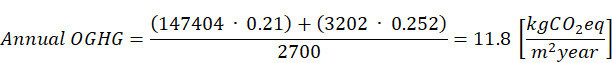
(50)
Based on the new score of the annual OGHG metric, S.3.1 score can be re-estimated in relation to the baseline metric score at EU level by using again Equation (35), as follows (Equation (51)):
(51)
However, the use of additional insulation material will increase the embodied energy and carbon of the envelope construction by an average of 90.7 MJ/kg of thermal insulation material that varies depending on the type of thermal insulation material (Dascalaki et al., 2020). Usually this additional embodied energy-carbon can be recovered in about 2-3 years because of operational savings, depending on the prevailing weather conditions and heating loads. Selecting thermal insulation material with a lower carbon footprint may reduce the overall embodied GHG emissions to 669060 kgCO2eq or 247.8 kgCO2eq/m2. This is close to the average value of global trends at 377 kgCO2eq/m2 (Röck et al., 2020). Residential buildings have reported values as low as 50 kgCO2eq/m2 (Röck et al., 2020). Similar targets are also set in ASHRAE Standard 100 (ASHRAE, 2024).
Based on this, the S.3.2 improvement is obtained by considering the use of insulation material with lower embodied carbon, assuming a score of the EGHG metric equal to 247.8 kgCO2eq/m2. Based on the new score of the EGHG metric, S.3.2 score can be re-estimated in relation to the baseline metric equal to the mean of embodied GHG emissions per unit floor area for new residential buildings (i.e. Tbaseline = 600 kgCO2eq/m2, according to Rock et al., 2022) by using again Equation (38), as follows (Equation (52)).
(52)
Based on the new scores of S.3.1 and S.3.2 indicators within the first scenario of improvement, S.3 can be estimaded again at the EU context, resulting into a score equal to 59.5 that corresponds to the Good performance class (Figure 22, newbuild/residential), as reported in Table 22.
Table 22. Example of S.3 evaluation (building scale) according to the first scenario of improvement of S.3.1 and S.3.2 score.
| EU context | ||
| Indicator | S.3.1 | S.3.2 |
| Indicator score | 60.7 | 58.7 |
| S.3 score | 0.4 • 60.7 + 0.6 • 58.7 = 59.5 | |
| S.3 performance class | Good | |
| S.3 performance class score (PCSS.3) | 70 | |
Source: JRC
The first scenario provides an effective improvement, as the KPI passed from the Acceptable to the Good performance class, also at EU level. However, building decarbonisation efforts and requirements mandate shifting from onsite combustion and the use of natural gas to the electrification of all building services; hence, a second scenario of improvement is considered in this direction.
The second scenario of improvement also relies on the S.3.1 and S.3.2 improvement. The S.3.1 improvement is achieved by using a heat pump with a high seasonal performance of about 3.6, instead of the natural gas boiler, reducing the final energy use for space heating and DHW to about 36,851 kWhe. The score of the annual operational GHG emissions metric related to heating, DHW, and cooling uses of the building is then re-estimated by using Equation (34), as follows (Equation (53)).
(53)
Based on the new score of the annual OGHG metric due to the electrification of the building, S.3.1 score can be re-estimated in relation to the baseline metric score at both Italian and EU level by using again Equation (35), as follows (Equation (54) and (55), respectively).
(54)
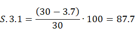
(55)
The S.3.2 improvement is the same considered for the first scenario, thus resulting equal to 58.7. Based on the new scores of S.3.1 and S.3.2 indicators, S.3 results into a score estimated equal to 71.9 or 70.3, depending on the Italian or EU context, that corresponds in both cases to the Excellent performance class (Figure 22, newbuild/residential), as reported in Table 23.
Table 23. Example of S.3 evaluation (building scale) according to the second scenario of improvement of S.3.1 and S.3.2 score.
| Italian context | ||
| Indicator | S.3.1 | S.3.2 |
| Indicator score | 91.7 | 58.7 |
| S.3 score | 0.4 • 91.7+ 0.6 • 58.7 = 71.9 | |
| S.3 performance class | Excellent | |
| S.3 performance class score (PCSS.3) | 100 | |
| EU context | ||
| Indicator | S.3.1 | S.3.2 |
| Indicator score | 87.7 | 58.7 |
| S.3 score | 0.4 • 87.7 + 0.6 • 58.7 = 70.3 | |
| S.3 performance class | Excellent | |
| S.3 performance class score (PCSS.3) | 100 | |
Source: JRC
3.7 Enhance sustainable mobility in the built environment (S.4)
3.7.1 Description and assessment
At building scale, enhance sustainable mobility in the built environment (S.4) KPI is assessed through the following two indicators:
- e-Mobility: electric vehicle (EV) parking (S.4.1).
- Alternative mobility: bicycle (S.4.2).
The S.4 score at building scale is evaluated according to Equation (56) using different indicator weights (wS.4.j) corresponding to the different combinations of the project classification according to type (i.e. newbuild or renovation)/main use (i.e. residential or non-residential) of a building scale project, as reported in Table 5. As example, the indicator weights within Equation (56) refer to a project classified as building scale, newbuild type, and residential main use.
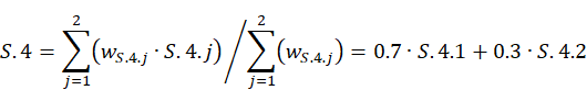
(56)
The S.4 KPI thresholds to associate the KPI score to the corresponding KPI performance class at building scale are illustrated in Figure 29.
Figure 29. S.4 performance classes and thresholds (building scale).

Source: JRC
At neighbourhood/urban scale, enhance sustainable mobility in the built environment (S.4) KPI is assessed through the following five indicators:
- e-Mobility: electric vehicle (EV) parking (S.4.1).
- Alternative mobility: bicycle (S.4.2).
- Public transportation systems – Extend (S.4.3).
- Public transportation systems – Usage (S.4.4).
- Public transportation systems – Accessibility (S.4.5).
S.4 score is evaluated according to Equation (57) using the different indicator weights (wS.4.j) corresponding to the different combinations of the project classification according to type (i.e. newbuild or renovation)/main use (i.e. residential or non-residential) of a neighbourhood/urban scale project, as reported in Table 5. As example, the indicator weights within Equation (57) refer to a project classified as neighbourhood scale, renovation type, and residential main use.
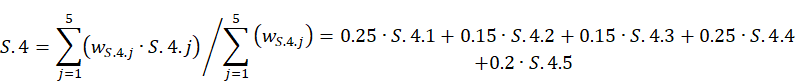
(57)
S.4 KPI thresholds to associate the KPI score to the corresponding KPI performance class at neighbourhood/urban scale are illustrated in Figure 30.
Figure 30. S.4 performance classes and thresholds (neighbourhood/urban scale).

Source: JRC.
3.7.2 e-Mobility: electric vehicles (EV) parking (S.4.1)
Electric vehicles are expected to play a crucial role in the decarbonisation and efficiency of the electricity system, through the provision of flexibility, balancing and storage services, especially through the development of smart charging and aggregation. The potential benefits of EVs to integrate with the electricity system and contribute to system efficiency and further absorption of renewable electricity can be exploited through the installation of a proper recharging infrastructure at building scale and the creation of public parking spaces with a recharging infrastructure at neighbourhood and urban scale.
At building scale, the e-Mobility: electric vehicle (EV) parking (S.4.1) indicator explores the EV-friendliness and availability of a parking facility in the form of car parking spaces serving a building to evaluate the proportion of car parking spaces with recharging points for EVs.
The S.4.1 score, which ranges between 0 and 100, is assessed according to a three-step framework that consecutively estimates the scores of specific sub-metrics and metrics to finally evaluate the indicator score, as follows:
- Number of parking spaces (NPS) sub-metric evaluation: the total number of car parking spaces serving a building are quantified. In line with the EPBD recast (Directive 2024/1275), a parking space is included into the counting if it is (i) inside the building, and/or (ii) physically adjacent to the building (i.e. a car parking space within the property area or in the direct vicinity of the building), and/or (iii) having a clear link with the building (e.g. a car parking space, not adjacent to the building, but identified to exclusively serve the building and reacheable through a dedicated shuttle bus service).
- Number of recharging points (NRP) sub-metric evaluation: the total number of car parking spaces with an EVrecharging point serving the building project needs to be quantified. Based on the NPS score, a parking space served by an EV-recharging point is included in the counting if the recharghing point has a power output higher than 3.7 kW (Regulation, 2023/1804). Beyond this condition, recarching points where EVs typically park for extended periods of time also need to be capable of smart recharching functionalities (Directive 2024/1275) to be included in the counting of NRP. Furthermore, each recharging point serves one electric vehicle at time.
- S.4.1 score evaluation: the metric regarding the share of car parking spaces with a recharging point for EVs over the total number of car parking spaces is estimated as the ratio of NRP (quantified in step 2) to NPS (quantified in step 1), expressed as a percentage. Subsequently, the S.4.1 score is estimated according to Equation (58) as a ratio, in which the numerator is the difference of the score of the aforementioned metric against a baseline metric (Tbaseline) score corresponding to the minimum required share of parking spaces equipped with a EV-recharging point, and the denominator is the same baseline metric score, multiplied by 100, so that the indicator score can be expressed as a dimensionless value that varies between 0 and 100.
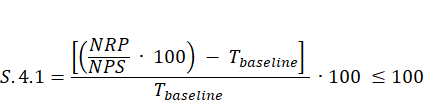 |
(58)
S.4.1 score indicates the extent to which the number of car parking spaces served by EV-recharching points over the total number of car parking spaces exceeds or subceeds the baseline value in relative terms. If the metric score is greater than the baseline metric score, S.4.1 score results into a positive value; noting though that the S.4.1 maximum score cannot exceed 100. If the metric score is lower than the baseline metric score leading the difference in the numerator to be negative, S.4.1 score results into a negative value pointing out that the indicator performance does not satisfy the baseline metric, thus the S.4.1 score is set equal to zero (0).
The score of the baseline metric (Tbaseline) to be used in Equation (58) is defined by national or local ordinances, or it can be set based on the rationale that a project at building scale should at least meet the EU minimum requirements for car parking spaces with EV-recharching points, according to Article 14 ‘Infrastructure for sustainable mobility’ of the recast EPBD (Directive 2024/1275), as summarised in Table 24.
Table 24 EU minimum requirements for baseline metric score correspondoing to number ofcar parking spaces with an EV-recharging pointin buildings, depending on building type/use and number of car parking spaces.
| Building use | Building type | Applicability threshold | EU minimum requirement for baseline value |
Non-residential (excluding office buildings) | Newbuild/renovation1 | > 5 parking spaces | At least 1 recharging point for every 5 parking space (20 %) |
Non-residential (including only office buildings) | New/renovation1 | > 5 parking spaces | At least 1 recharging point for every 2 parking space (50 %) |
| Non-residential buildings | Newbuild/renovation | > 20 parking spaces | At least 1 recharging point for every 10 parking space (10 % |
| Residential | Newbuild/ renovation1 | > 3 parking spaces | At least 1 recharging point for every 3 parking space (33 %) |
1 According to the 2024 recast EPBD, in this case renovation is intended as major renovation
Source: JRC; data from EPBD (Directive, 2024/1275)
At neighbourhood/urban scale, the e-Mobility: electric vehicle (EV) parking (S.4.1) indicator addresses the availability of public car parking facilities within the project area by evaluating the proportion of car parking spaces served by a recharging point for EVs.
S.4.1 score, which ranges between 0 and 100, is assessed according to the following three-step framework that consecutively estimates the scores of sub-metrics and metrics to finally evaluate the indicator score:
- Number of recharging spaces (NRS) sub-metric evaluation: the total number of EV recharging stations within the neighbourhood/urban area are quantified. A recharging station is included into the counting only if its recharging points have a power output greater than 3.7 kW (Regulation, 2023/1804).
- Number of electric vehicles (NEV) sub-metric evaluation: the total number of electric vehicles registered within the neighbourhood/urban area. is quantified:
- S.4.1 score evaluation: the metric concerning the number of EV-recharging stations per registered electric vehicle, is estimated as the ratio of NRS (quantified in the step 1) to NEV (quantified in the step 2), expressed as a percentage. Subsequently, the S.4.1 score is estimated, according to Equation (59), as a ratio in which the numerator is the difference of the score of the aforementioned metric against the score of the baseline metric (Tbaseline) of the public car parking facilities equipped with a recharging station for EVs and the denominator is the score of the same baseline metric, multiplied by 100, so that S.4.1 score can be expressed as a dimensionless value that varies between 0 and 100.
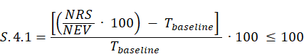
(59)
S.4.1 can also be assessed against a baseline that is set at a value representing the existing status at the beginning of the project. If the metric score is greater than the reference baseline value, S.4.1 score results into is positive value; noting though that the S.4.1 maximum score cannot exceed 100. If the metric score is lower than the reference baseline value leading the difference in the numerator to be negative, S.4.1 score assumes a negative value indicating that the indicator performance does not satisfy the reference baseline, thus S.4.1 score is set equal to zero (0).
The score of the baseline metric in Equation (59) can be set based on the rationale that a neighbourhood/urban scale project should at least meet the local or national minimum requirements for EV‑recharging stations to facilitate the alternative mobility plans and the use of EVs. The mandatory national fleet based target for publicly available electric recharging infrastructure for light duty road vehicles (i.e. cars and vans) is at least 1.3 kW for every battery electric vehicle and for every plug-in hybrid light-duty vehicle, and a total power output of at least 0.8 kW must be provided through publicly accessible recharging stations (Regulation, 2023/1804). In addition, EU Member States shall ensure that recharging stations are in place for heavy-duty vehicles in urban nodes and in safe and secure parklings. The number of electric light-duty vehicles per public EV charging point varies from about 2 vehicles per charging point in Korea to almost 100 in New Zealand, while the EU average public charging power capacity per light duty vehicle is 1.2 kW per EV (IEA, 2023).
3.7.3 Alternative mobility: bicycle (S.4.2)
The availability of bicycle parking spaces for new and majorly renovated buildings in the EU has been introduced as a design key-feature to remove barriers to cycling as a central element of a sustainable and zero-emission mobility (Directive 2024/1275). Bicycle parking spaces of a building project can be indoor or outdoor, depending on their location inside the building or in an area, if available, belonging to the building, but placed outside it.
Furthermore, the creation of connected networks of physically protected bicycle lanes at neighbourhood and urban scale, rather than individual or unprotected lanes, is generally regarded as the most important factor in promoting cycling. At building scale, the alternative mobility: bicycle (S.4.2) indicator assesses the proportion of indoor and/or outdoor bicycle parking spacesof a building project in relation to building users (i.e. number of building occupants), as for non-residential buildings, or in relation to the number of dwellings, as for residential buildings.
The S.4.2 score, which ranges between 0 and 100, is assessed according to a three-step framework that consecutively estimates the scores of specific sub-metrics and metrics, which are evaluated differently based on the project classification according to use (i.e. residential or non-residential), to finally evaluate the indicator score, as follows:
- Number of bicycle parking spaces (NBPS) sub-metric evaluation: the total number of available indoor and/or outdoor bicycle parking spaces of a building project needs to be quantified. This information can be verified from design documents in case of newbuild projects or from on-site inspection in case of renovation project of existing buildings.
User capacity (UC) of building or Number of dwellings (NDW) sub-metric evaluation: the user capacity of building sub-metric is considered for non-residential building projects, whereas the number of dwelling sub-metric is used for residential building projects, thus the evaluation of each sub-metric is carried out, as follows:
a) Non-residential building: the total user capacity of a building project, including both employees and visitors (if applicable), is quantified by retrieving relevant data from the building design documents, as for newbuild projects, or by using statistical data, as for renovation projects of existing buildings, if a registry is available
b) Residential building: the total number of dwellings is quantified by usingthe building design documents, as for newbuild projects, or a building survey, as for renovation projects of existing buildings.
S.4.2 score evaluation: the indicator score evaluation varies depening on the building project classification according to use, as follows:
a) Non-residential building: the metric regarding the number of bicycle parking spaces per user capacity of a building is estimated as the ratio of NBPS (quantified in step 1) to UC (quantified in step 2), expressed as a percentage. Subsequently, the S.4.2 score is evaluated according to Equation (60) as a ratio, in which the numerator is the difference of the aforementioned metric score against the score of a baseline metric (Tbaseline) of bicycle parking spaces and the denominator is the same baseline metric score, multiplied by 100, so that the indicator score can be expressed as a dimensionless value that varies between 0 and 100.

(60)
S.4.2 score indicates the extent to which the number of bicycle parking spaces per user capacity exceeds or subseeds the reference baseline value. If the metric score is greater than the baseline metric score, S.4.2 score results into a positive value; noting though that the indicator maximum score cannot exceed 100. If the metric score is lower than the score of the baseline metric leading to a negative difference in the numerator, S.4.2 results into a negative score indicating that the building performance does not satisfy the baseline metric, thus S.4.1 score is set equal to zero (0).
b) Residential buildings: the metric regarding the share of bicycle parking spaces over the number of dwellings is estimated as the ratio of NBPS (quantified in step 1) to ND (quantified in step 2 expressed as a percentage. Subsequently, the S.4.2 score is estimated according to Equation (61) as a ratio, in which the numerator is the difference of the aforementioned metric score against the score of a baseline metric (Tbaseline) corresponding to the minimum required share of bicycle parking spaces and the denominator is the score of the same baselinemetric, multiplied by 100, so as the indicator score can be expressed as a dimensionless value that varies between 0 and 100.
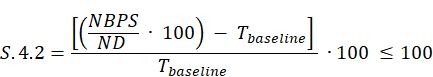 |
(61)
If the metric score is higherer than the baselinemetric score, S.4.2 score results into a positive value, noting though that the indicator maximum score cannot exceeds 100. If the metric score is lower than the baseline metric score leading the difference in the numerator to be a negative value, S.4.2 score points out that the indicator performance does not satisfy the baseline metric and S.4.2 score is set equal to zero (0).
The scores of the baseline metric to be used in Equation (60) and (61) are defined by national or local ordinances. Alternatively, they can be set based on the rationale that a project at building scale should at least meet the EU minimum requirements for bicycle parking spaces, according to Article 14 ‘Infrastructure for sustainable mobility’ of the recast EPBD (Directive 2024/1275), as summarised in Table 25.
Table 25. EU minimum requirements for baseline metric scorecorresponding to bicycle parking spaces per user capacity or per dwelling in buildings, depending on building type/use and number of car parking spaces.
| Building use | Building type | Applicability threshold | Minimum requirements for baseline metric |
Residential
| Newbuild | > 3 car parking spaces
| 2 bicycle parking spaces for every dwelling |
| Renovation1 | 2 bicycle parking spaces for every dwelling If the above is not technologically and economically feasible, ensure as many bicycle parking spaces as appropriate | ||
| Non-residential | Newbuild/renovation1 | > 5 car parking spaces | Bicycle parking spaces representing at least 15 % of the average or 10 % of user capacity of the building |
| Non-residential buildings | Newbuild/renovation | > 20 car parking spaces | Bicycle parking spaces representing at least 15% of the average or 10 % of user capacity of the building |
1 According to the 2024 EPBD recast, in this case renovation refer to as a major renovation.
Source: JRC; data from EPBD (Directive, 2024/1275)
At neighbourhood/urban scale, the alternative mobility: bicycle (S.4.2) indicator evaluates the extension of the bicycle paths-lanes network in relation to the inhabitants of the designated project area and provides a useful measure of a diversified transportation system according to ISO 37120 (ISO, 2018).
The S.4.2 score, which ranges between 0 and 100, is assessed according to a three-step framework that consecutively estimates the scores of specific sub-metrics and metrics to finally evaluate the indicator score, as follows:
- Length of bicycle paths and lanes (LBPL) sub-metric evaluation: the total length (expressed in kilometres) of the available bicycle paths and lanes in a neighbourhood/urban scale project with a minimum width of a one-way bicycle lane equal to 1.5 m is estimated considering a recommended width equal to 2 m to provide enough space for cyclists to ride side by side and pass each other safely (ISO, 2018). The width of bicycle paths varies depending on the intended use and expected traffic volume but should be wide enough to accommodate two-way bicycle traffic, ranging from 2 to 3 m (ISO, 2018).
- Population (P) sub-metric evaluation: the total number of inhabitants within the area of the neighbourhood or urban scale project is quantified, depending on the physical boundary of the project area.
- S.4.2 score evaluation: the metric concerning the length of bicycle paths and lanes per 1000 inhabitants is estimated as the ratio of LBPL (quantified in step 1) to one 1000th of (P) (quantified in step 2), expressed as the kilometres of bicycle paths and lanes per 1000th inhabitants. Subsequntly, S.4.2 score is evaluated according to Equation (62) as a ratio, in which the numerator is the difference of the score of the aforementioned metric against the score of a baseline metric (Tbaseline) of the bicycle paths and lanes length per 1000 inhabitants and the denominator is the score of the same baseline metric, multiplied by 100, so that the indicator score varies between 0 and 100.
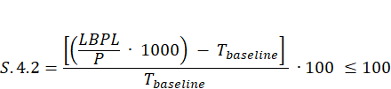 |
(62)
If the metric score is greater than the baseline metric score, S.4.2 score results into a positive value, noting though that the indicatormaximum score cannot exceed 100. If the metric score is lower than the score of the baseline metric leading to a negative difference in the numerator, S.4.2 score indicates that the indicator performance does not satisfy the baseline metric and S.4.2 score is set equal to zero (0).
The score of the baseline metric (Tbaseline) in Equation (62) can be set based on the rationale that a neighbourhood/urban scale project should at least meet the local or national minimum requirements for bicycle paths and lanes length. However, an average value of 0.15 km/1000 inhabitants (Eurostat, 2021) can be also assumed as the score of the baseline metric. Another option to set this score takes into account the best practices of bicycle paths and lanes length per 1000 inhabitants (Wolniak 2023). Specifically, a reference best practice is currently set at 7.8 km/1000 inhabitants in Finland, followed by Sweden (3.24 km/1000 inhabitants), Luxembourg (1.39 km/1000 inhabitants), Germany (1.59 km/1000 inhabitants) and Hungary (1.18 km/1000 inhabitants).
3.7.4 Public transportation systems: extend (S.4.3)
The public transportation systems: extend (S.4.3) indicator is considered exclusively at neighbourhood/urban scale to evaluate the extension of the public transportation network in relation to the population within the area of a neighbourhood or urban scale project, according to ISO 37120 (ISO, 2018). Cities with larger amounts of public transport might tend to be more geographically compact and supportive than areas relying on non-motorised modes of transportation. It is essential to evaluate the S.4.3 indicator along with the other two indicators relevant to the public transportation systems (i.e. S.4.4 and S.4.5, respectively concerning the usage and accessibility aspects) to identify an overall picture of the strengths and weaknesses of the public transportation systems within a neighbourhood/urban scale project.
The S.4.3 score, which ranges between 0 and 100, is assessed according to a three-step framework that estimates the scores of specific sub-metrics and metrics consecutively to finally evaluate the indicator score, as follows:
- Length of public transport systems (LPT) sub-metric evaluation: the length of route (expressed in Km) covered by public transport systems operating within the area of the neighbourhood or urban scale projectis estimated. Public transport shall include both high capacity systems (i.e. rail metro, subway systems, commuter rail) and low capacity systems i.e. Bus Rapid Transit (BRT) systems, light rail, streetcars/tramways, buses, trolleybuses). Other passenger transport services may also be included. Data from each type of transport system can be included and listed individually to document the kilometres of public transport by system type. If different public transport systems cover a same route, the length shall be counted for each transport system (e.g if a bus and a streetcar cover the same 1-km route, the length of the public transport systems counts for 2 km). Relevant data should be gathered from municipal transport offices and local/regional transit authorities and can also be counted using computerised mapping, aerial photography or existing paper maps, all of which shall be field verified. This information may be gathered from transport system plans or other master plans.
- Population (P) sub-metric evaluation: the total number of inhabitants within the area of the neighbourhood or urban scale project is quantified by using available statistical data.
- S.4.3 score evaluation: the metric concerning the total length, in kilometres, of the public transport system within the neighbourhood/urban area per 10 000 inhabitants is assessed as the ratio of LPT (quantified in step 1) to one 10 000th of P (quantified in step 2). Subsequently, the S.4.3 score is estimated according to Equation (63) as a ratio, in which the numerator is the difference of the score of the aforementioned metric against the score of a baseline metric (Tbaseline) of the total length of public transport systems per 10 000 inhabitant and the denominator is the score of the same baseline metric, multiplied by 100, so that the indicator score varies between 0 and 100.
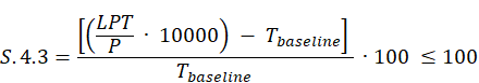
(63)
If the metric score is greater than the baseline metric score, S.4.3 score results into a positive value, noting though that the S.4.3 maximum score cannot exceed 100. If the metric score is lower than the baseline metric score, leading the difference in the numerator to be negative, S.4.3 score results into a negative value pointing out that the indicator performance does not satisfy the baseline metric and S.4.3 score is set equal to zero (0).
The score of the baseline metric (Tbaseline) to be used in Equation (63) can be set based on the rationale that a neighbourhood/urban scale project should at least meet the minimum local or regional requirements for the total length of public transport systems (expressed in kilometers) per 10 000 inhabitants. The baseline value to evaluate the indicator may take its value at time zero, when the project objectives are established. Another option to set the score of the baseline metric refers to relevant standardised city data on the length of high and low capacity systems per inhabitants provided for 56 European cities by the Open Data Portal of the World Council on City Data (WCCD)[1], which is based on ISO 37120 (ISO, 2018). Representative data for some European cities are reported in Table 26.
Table 26. Baseline metric score corresponding to the total length of public transport systems (in km) per 10 000 inhabitants of representative European cities
| City/Country | City population (inhabitants) | City land area (km2) | Length of public transport systems (in km) per 10 000 inhabitants1, as baseline metric | ||
| High capacity systems | Low capacity systems | Total | |||
| Amsterdam (The Netherlands) | 834 713 | 164.66 | 1.44 | 2.63 | 4.07 |
| Barcelona (Spain) | 1 611 822 | 102.16 | 1.59 | 5.82 | 7.41 |
| Eindhoven (The Netherlands) | 224 788 | 88.84 | 0.09 | 5.21 | 5.3 |
| Gdynia (Poland) | 247 478 | 135.00 | 0.44 | 9.78 | 10.22 |
| Heerlen (The Netherlands) | 87 406 | 45.53 | 1.15 | 11.44 | 12.59 |
| Kielce (Poland) | 197 704 | 110.00 | 1.16 | 67.09 | 68.25 |
| Koprivnica (Croatia) | 30 872 | 90.94 | 0 | 2.59 | 2.59 |
| London (UK) | 8 538 700 | 1,572 | 1.43 | 4.51 | 5.94 |
| Porto (Portugal) | 214 329 | 41.42 | 1.89 | 28.91 | 30.8 |
| Rotterdam (The Netherlands) | 618 357 | 208.88 | 1.34 | 1.60 | 2.94 |
| Sintra (Portugal) | 382 521 | 319.23 | 0.81 | 50.21 | 51.02 |
| The Hague (The Netherlands) | 519 988 | 98.13 | 0.36 | 2.28 | 2.64 |
| Valencia (Spain) | 787 266 | 137.48 | 1.44 | 5.87 | 7.31 |
| Zagreb (Croatia) | 790 017 | 641.32 | 0.33 | 20.01 | 20.34 |
| Zwolle (The Netherlands) | 124 896 | 119.3 | 4.65 | 0.15 | 4.8 |
1 Data based on WCCD.
Source: adapted from Hajduk, 2022.
[1] . World Council on City Data (WCCD), https://www.dataforcities.org
3.7.5 Public transportation systems: usage (S.4.4)
The public transportation systems: usage (S.4.4) indicator is considered exclusively for neighbourhood/urban scale projects to evaluate the usage of the public transportation network in relation to the population within the designated neighbourhood or urban area, according to ISO 37120 (ISO, 2018). Cities with higher transport ridership rates tend to invest more in their transport systems, also becoming more geographically compact. The transport usage does not focus exclusively on pupulation’s journeys to reach the work place, but it addresses the overall travel patterns in a city. This also provides insight into transportation policy, traffic congestion, accessibility and urban form. It is essential to evaluate the S.4.4 indicator along with the other two indicators relevant to the public transportation systems (i.e. S.4.3 and S.4.5 concerning the extend and accessibility aspects, respectively) to identify an overall picture of the strengths and weaknesses of the public transportation systems within a neighbourhood/urban scale project.
The S.4.4 score, which ranges between 0 and 100, is assessed according to a three-step framework that estimates the scores of specific sub-metrics and metrics consecutively to finally evaluate the indicator score, as follows:
Number of public transport trips (NPTT) sub-metric evaluation: the total annual number of public transport trips originating in area of the neighbourhood/urban scale project are determined. Public transport trips shall include trips via high capacity systems (i.e. heavy rail metro or subway, commuter rail) and low capacity systems (i.e. light rail, streetcars and tramways, bus, trolleybus) and other public transport services may also be included. Transport systems often serve entire metropolitan areas, and not just central cities. Public transport data should be gathered from a number of sources including municipal transport authorities, official transport surveys, revenue collection systems (e.g. number of fares purchased) and national censuses.
The use of number of public transport trips with origins in the city itself will capture many trips whose destination is outside the city, but will generally capture the impact that the city has on the regional transport network. Trips made via “informal transport” services (e.g. minibuses not operated by the government or municipal transport corporation) shall not be counted because they are not part of the official transport network.
5. Population (P) sub-metric evaluation: the total number of inhabitants within a neighbourhood or urban area is quantified by using available statistical data.
6. S.4.4 score evaluation: based on the sub-metric scores above, the metric evaluating the annual number of public transport trips originating in area of the neighbourhood/urban scale project per capita, i.e. ‘ridership of public transport’, is estimated as the ratio of NPTT (quantified in step 1) to P (quantified in step 2). Subsequently, the S.4.4 score is estimated according to Equation (64) as a ratio, in which the numerator is the difference of the score of the aforementioned metric against the score of a baseline metric (Tbaseline) of the public transport trips per capita and the denominator is the reference score of the same baseline metric, multiplied by 100, so that the indicator score varies between 0 and 100.
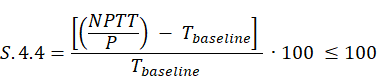
(64)
If the metric is greater than the score of the baseline metric, S.4.4 score results into a positive value, noting though that the S.4.3 maximum score cannot exceed 100. If the metric score is lower than the score of the baseline metric, leading the difference in the numerator to be negative, S.4.4 results into a negative score pointing out that the performance does not satisfy the baseline metric, thus S.4.4 score is set equal to zero (0).
The score of the baseline metric (Tbaseline) to be used in Equation (64) can be set based on the rationale that a neighbourhood/urban scale project should at least meet the minimum requirements for the annual total public transport trips per capita. The baseline value to evaluate the indicator may take its value at time zero, when the performance objectives concerning the use of public transportation are established. Similarly to the S.4.3 indicator, another option to set the score of the baseline metric refers to relevant standardised city data on annual number of public transport trips per capita provided for 56 European cities by the Open Data Portal of the World Council on City Data (WCCD)[1], which is based on ISO 37120 (ISO, 2018), as reported for some representative European cities in Table 27.
Table 27. Baseline metric score corresponding to the total number of public transport trips per capita of representative European cities.
| City/Country | City population | City land area (km2) | Annual number of public transport trips per capita1, as baseline metric |
| Amsterdam (The Netherlands) | 834 713 | 164.66 | 265 |
| Barcelona (Spain) | 1 611 822 | 102.16 | 442 |
| Eindhoven (The Netherlands) | 224 788 | 88.84 | 190 |
| Gdynia (Poland) | 247 478 | 135.00 | 240 |
| Heerlen (The Netherlands) | 87 406 | 45.53 | 65 |
| Kielce (Poland) | 197 704 | 110.00 | 177 |
| London (UK) | 8 538 700 | 1572 | 490 |
| Porto (Portugal) | 214 329 | 41.42 | 637 |
| Rotterdam (The Netherlands) | 618 357 | 208.88 | 248 |
| Sintra (Portugal) | 382 521 | 319.23 | 44 |
| The Hague (The Netherlands) | 519 988 | 98.13 | 111 |
| Valencia (Spain) | 787 266 | 137.48 | 159 |
| Zagreb (Croatia) | 790 017 | 641.32 | 343 |
| Zwolle (The Netherlands) | 124 896 | 119.3 | 56 |
1 Data based on WCCD.
Source: Hajduk, 2022
3.7.6 Public transportation systems: accessibility (S.4.5)
The public transportation systems: accessibility (S.4.5) indicator is considered exclusively for neighbourhood/urban scale projects to evaluate the accessibility of the public transportation network in relation to the population within the area of the neighbourhood or urban scale project, according to ISO 37120 (ISO, 2018) and in line with the UN SDG indicator 11.2.1. Proximity to reliable and connected public transport provides the essential basis to larger share the public transit mode thus reducing congestion and other externalities. Greater transportation options also improve the liveability of cities.This also provides insight into transportation policy, traffic congestion, accessibility and urban form.
The S.4.5 score, which ranges between 0 and 100, is assessed according to a three-step framework that estimates the scores of specific sub-metrics and metrics consecutively to finally evaluate the indicator score, as follows:
- Number of inhabitants (NI) sub-metric evaluation the total number of inhabitants, within the area of the neighbourhood or urban scale project, that live within 0.5 km of public transit running at least every 20 min during peak periods is determined. Peak periods are intended as the two 3-hour periods in a day when the traffic volume is highest; usually occurring one in the morning and the other in the evening.Generally, peak periods differ by region and municipality. Comprehensive data on the location of public transport stops, a complete street network, and data on the spatial distribution of inhabitants within the area of the neighbourhood or urban scale project need to be collected. Data shall be in the form of GIS layers, which are usually made available by local or regional authorities. Schedules of public transit are available from municipal public transportation operators. The georeferenced population census can be derived by relating the inhabitants in the area with their address in the georeferenced municipal street guide. The result will be a point layer in which each point represents one person’s place of residence. Therefore, there would be as many points as there are inhabitants. Once both layers, transit stops and georeferenced population, are included in the GIS, proximity buffers of the transit stops (500 m radius) shall be created with the help of the GIS buffer geoprocess.
- Population (P) sub-metric evaluation: the total number of inhabitants within the neighbourhood or urban area is quantified by using available statistical data.
- S.4.5 score evaluation: the metric concerning the share of inhabitants living within 0.5 km of public transit running at least every 20 min during peak periods over the total number of inhabitants within the neighbourhood or urban area is estimated as the ratio of NI (quantified in step 1) to P (quantified in step 2), expressed as percentage. Subsequently, S.4.5 score is assessed according to Equation (65) as a ratio, in which the numerator is the difference of the score of the aforementioned metric against the score of a baseline metric (Tbaseline) of the total number of inhabitants living within 0.5 km of public transit running at least every 20 min during peak periods and the denominator is the score of the same the baseline metric, multiplied by 100, so as the indicator score can be expressed as a dimensionless value that varies between 0 and 100.
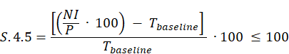
(65)
If the metric score is greater than the baseline metric score, S.4.5 results into a positive score, noting though that the indicator maximum score cannot exceed 100. If the metric score is lower than the score of the baseline metric, leading the difference in the numerator to be negative, S.4.5 results into a negative score demonstrating that the indicator performance does not satisfy the baseleine metric, thus the indicator score is set equal to zero (0).
The score of the baseline metric (Tbaseline) to be used in Equation (65) can be set based on the rationale that a neighbourhood/urban scale project should at least meet the minimum local or regional requirements for the inhabitants’ accessibility to the public transportation network. The access to a public transport stop within a 500 meters walking distance, regardless of the foreseen frequency of the public transport service at that stop, is usually not a critical issue for most of the population in urban centres of European cities, according to a study by Poelman et al. (2020) measuring the proportion of population that has convenient access to public transport in line with the UN SDG indicator 11.2.1[1]. This study provides results for 685 urban centres in EU-27, EFTA countries and the United Kingdom, pointing out that, in more than 45 % of the cities reviewed, the share of population with access to a nearby stop exceeds 95 %. However, this figure could lower, since the frequency of the public transport service is taken into account; a recommended score for the baseline metric in Equation (65) is assumed equal to 90 %.
[1] UN SDG indicator 11.2.1: ‘Proportion of population that has convenient access to public transport, by sex, age and people with disabilities’, https://unstats.un.org/sdgs/metadata/files/Metadata-11-02-01.pdf
3.7.7 Example (S.4)
The example for the evaluation of the S.4 KPI is carried out by considering two projects referring to a building and an urban scale project, respectively.
The building scale project is a new naturally ventilated multifamily residential building with a useful internal floor area of 2700 m2, located in Turin (Italy). The building features a total amount of 22 car parking spaces: all of them have pre-cabling to enable the installation of recharging points for EVs, while ten out of the 22 parking spaces have installed recharging points for EVs with a power output greater than 3.7 kW. The building is also served by 10 bicycle parking spaces.
The evaluation of the S.4 KPI at building scale to enhance the building characteristics related to sustainable mobilitydepends on the scores S.4.1 and S.4.2 indicators.
The S.4.1 score is evaluated according to the three-step framework, as reported in Section 3.7.2, leading to the estimation of the scores of the sub-metrics and metrics to finally evaluate the indicator score, as follows:
- Number of parking spaces (NPS) sub-metric evaluation: the total number of car parking spaces is equal to 22.
- Number of recharging points (NRP) sub-metric evaluation: Out of the 22 car parking spaces, a total number of ten car parking spaces have recharging points for EVs with a power output higher than 3.7 kW.
S.4.1 score evaluation: the metric score estimated as the ratio of NRP (i.e. total number of car parking spaces with a recharging point, quantified in step 2) to NPS (i.e. total number of car parking spaces, quantified in step 1), is compared against the score of the baseline metric (Tbaseline). Specifically, the Tbaseline score is estimated according to the EU minimum requirement of one recharging point for every three car parking spaces by using data in Table 15, as the building scale project is classified as newbuild/residential/with more than three parking spaces. Hence, the minimum requirement for a new multifamily building with 22 car parking spaces corresponds to a total of 7 recharging points, which translates to a Tbaseline score of 31.8%. Having evaluated the NPS and NRP sub-metric scores and the baseline metric score, the S.4.1 score is evaluated using Equation (58), as follows (Equation (66)).
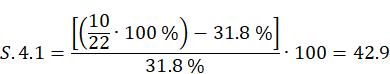
(66)
The indicator score is above the baseline of 31.8 %, so the result is positive and can be considered in the KPI assessment.
The S.4.2 score is evaluated according to the three-step framework, as reported in Section 3.7.3, leading to the estimation of the scores of specific sub-metrics and metrics related to residential buildings, to finally evaluate the indicator score, as follows:
1. Number of bicycle parking spaces (NBPS) sub-metric evaluation: the total number of bicycle parking spaces serving the building is assumed equal to 10.
2. Number of dwellings (ND) sub-metric evaluation: the residential building consists of a total number of 22 dwellings.
3. S.4.2 score evaluation: the metric score estimated as the ratio of NBPS (quantified in step 1) to ND (quantified in step 2) is compared against the score of the baseline metric. Specifically, the Tbaseline score is estimated according to the EU minimum requirement of 2 bicycle parking spaces for every dwelling by using data in Table 25, as the building scale project is classified as newbuild/residential and has more than three car parking spaces. Hence, the building scale project should have a minimum total number of bicycle parking spaces (NBPSmin) equal to 44, as the building project accounts for 22 dwellings, leading to a Tbaseline metric score equal to 200 %, according to Equation (67).
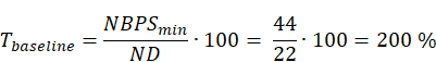
(67)
Having evaluated the NBPS and ND sub-metric scores and the baseline metric score, S.4.2 score is evaluated using Equation (61), as follows (Equation (68)). As expected, the indicator score is negative, as the number of bicycle parking spaces per dwelling is lower than the baseline metric score. Hence, S.4.2 score is set equal to zero (0).
(68)
Having evaluated the scores of S.4.1 and S.4.2 indicators, S.4 score is evaluated by using Equation (56) and considering the indicator weights corresponding to the combination of the project classification as building scale, newbuild type, and residential main use (Table 5). Hence, S.4 results into a score estimated equal to 30 that corresponds to the Low performance class (Figure 29, newbuild/residential), as reported in Table 28.
Table 28. Example of S.4 evaluation (building scale).
| Indicator | S.4.1 | S.4.2 |
| Indicator score | 42.9 | 0 |
| S.4 score | 0.7 • 42.9 + 0.3 • 0 = 30 | |
| S.4 performance class | Low | |
| S.4 performance class score (PCSS.4) | 25 | |
Source: JRC
The S.4 KPI can attain a performance class higher than Low by increasing both the number of car parking spaces with EV-recharging point and bicycle parking spaces per dwelling. Considering a project scenario for which all 22 parking spaces in the building scale project have installed recharging points for EVs and three bicycle parking spaces for every dwelling are ensured leading to a total number of bicycle parking spaces equal to 66, then the scores of S.4.1 and S.4.2 indicators are estimated equal to 100 and 50, respectively, according to Equation (69) and (70). S.4.1 score indicates that the number of car parking spaces with EV-recharging point exceeds the baseline score leading to a score greater than 100. However, the indicator score is set equal to its maximum score that is 100.
(69)
(70)
Based on the new scores of S.4.1 and S.4.2 indicators, S.4 results into a score estimated equal to 50 that corresponds to the Excellent performance class (Figure 29, newbuild/residential), as reported in Table 29.
Table 29. Example of S.4 evaluation (building scale) following the improvement of indicator scores
| Indicator | S.4.1 | S.4.2 |
| Indicator score | 100 | 50 |
| S.4 score | 0.7 • 100 + 0.3 • 50 = 85 | |
| S.4 performance class | Excellent | |
| S.4 performance class score (PCSS.4) | 100 | |
Source: JRC.
The neighbourhood/urban scale project refers to the renovation of a whole urban area, located in Turin (Italy), including a total amount of 55 public electric car recharging stations equipped with recharging points with a power output greater than 3.7 kW is considered. The number of electric cars registered in the designated urban area equals 1025, while the current local minimum requirements for public car parking facilities equipped with a recharging station is set at 3%. The urban area supports the alternative mobility providing bicycle paths and lanes for a total length of 121 km, according to the data provided by the Municipal Department of Transportation. The total population of the city is estimated equal to 723 540 inhabitants, according to the municipality records. Finally, the urban area is served by various high and low-capacity public transportation systems, which do not include a subway system, according to data provided by the Municipal Department of Transportation, as reported in Table 30. The same table also reports data on the total length of each public transportation system and the corresponding annual trips. The accessibility of the public transportation network is assessed using a geoportal platform. Currently, the local baseline metric score for the total length of public transport systems in the area is 5.3 km/10000 inhabitants, which compares well with other major European cities given in Table 26, and the local baseline metric score for the annual public transport trips in the area is 121 trips per capita.
Table 30. Example (S.4): public transportation systems within the area of the urban scale project.
| Public transportation system | Type of public transportation system | Total length (km) | Annual number of public transport trips originating in the area per transportation mode (million trips) |
| High-capacity systems | Heavy rail metro | 115 | 20 |
| Subway | 0 | 0 | |
| Commuter rail | 29 | 12 | |
| Total (high-capacity systems) | 144 | 32 | |
| Low-cpacity systems | Light rail | 180 | 4 |
| Streetcars / Tramways | 120 | 2 | |
| Busses and trolleybuses | 135 | 48 | |
| Bus rapid transit (BRT) | 145 | 16 | |
| Total (low-capacity systems) | 580 | 70 | |
| Total (high- and low-capacity systems) | 724 | 102 | |
Source: JRC.
The evaluation of the S.4 KPI at neighbourhood/urban scale depends on the scores of S.4.1, S.4.2, S.4.3, S.4.4 and S.4.5 indicators.
The S.4.1 score is evaluated according to the three-step framework reported in Section 3.7.2, leading to the estimation of the scores of the sub-metrics and metrics to finally evaluate the indicator score, as follows:
- Number of recharging stations (NRS) sub-metric evaluation: the total number of recharging stations for EVs in the designated urban area is equal to 55.
- Number of electric vehicles (NEV) sub-metric evaluation: a total number of 1025 electric cars are registered in thedesignated urban area.
S.4.1 score evaluation: the metric score, estimated as the ratio of NRS (quantified in step 1) to NEV (quantified in step 2), leading to the share of recharching stations per EV, is compared against the score of the baseline metric (Tbaseline) for the area that is currently at 3 %. Considering the growth of electrification in transportation and the number of EVs in the city, there has been a strong effort to expand the public recharging stations. Having evaluated the NRS and NEV sub-metric scores and the baseline metric score, S.4.1 score is evaluated using Equation (59), as follows (Equation (71)).
(71)
Doubling the number of public recharging stations is significant progress, but will need more stations throughout the area to continue serving the growing number of EVs.
The S.4.2 score is evaluated according to the three-step framework reported in Section 3.7.3, leading to the estimation of the scores of the sub-metrics and metrics to finally evaluate the indicator score, as follows:
- Length of bicycle paths and lanes (LBPL) sub-metric evaluation: the total length of the available bicycle paths and lanes in the urban area with a width not less than 1.5 m is reported at about 121 km.
- Population (P) sub-metric evaluation: the total number of inhabitants within the urban area is estimated equal to 723 540
- S.4.2 score evaluation: the metric score evaluated as the ratio of LBPL (quantified in step 1) per one 1000th of P (quantified in step 2), leading to the length of bicycle paths and lanes in km per 1000 inhabitants, is compared against the score of the baseline metric (Tbaseline). Specifically, the Tbaseline score of the length of bicycle paths and lanes in km per 1000 inhabitants is assumed equal to the EU average of 0.15 km/1000 inhabitants. A value of 0.5 km/1000th inhabitants represents a well-developed bicycle network, so there is room for expanding and improving the bicycle paths and lanes in the area.
Having evaluated the LBPL and P sub-metric scores and the baseline metric score, S.4.2 score is evaluated using Equation (62), as follows (Equation (72)).
(72)
The S.4.3 score is evaluated according to the three-step framework reported in Section 3.7.4, leading to the estimation of the scores of the sub-metrics and metrics to finally evaluate the indicator score, as follows
- Length of public transport systems (LPT) sub-metric evaluation: the total length of routes covered by public transport systems, operating within the area of the urban scale project, is estimated equal to 724 km (Table 30).
- Population (P) sub-metric evaluation:the total number of inhabitants within the area of the urban scale project is reported at 723 540.
S.4.3 score evaluation: the metric score evaluated as the ratio of LPT (quantified in step 1) to one 10000th of P (quantified in step 2), leading to the length of public transport system in km per 10000 inhabitants, is compared against the score of the local baseline metric (Tbaseline) that is currently at 5.3 km/10000 inhabitants for the area. Having evaluated the LPT and P sub-metric scores and using the local baseline metric score, S.4.3 score is evaluated using Equation (63), as follows (Equation (73)).
(73)
The S.4.4 score is evaluated according to the three-step framework reported in Section 3.7.5, leading to the estimation of the scores of the sub-metrics and metrics to finally evaluate the indicator score, as follows:
1. Number of public transport trips (NPTT) sub-metric evaluation: the annual total number of trips operating within the area of the urban scale project is 102 million (Table 30).
2. Population sub-metric evaluation: the total number of inhabitants in the area of the urban scale project is reported at 723 540.
3. S.4.4 score evaluation: the metric score estimated as the ratio of NPTT (quantified in step 1) to P (quantified in step 2), leading to the number of public transport trips per capita, is compared against the score of the baseline metric (Tbaseline) at local level that is currently equal to 121 annual public transport trips per capita for the area. Having evaluated the NPTT and P sub-metric scores and the baseline metric score, S.4.4 score is evaluated using Equation (64), as follows (Equation (74)).
(74)
The S.4.5 score is evaluated according to the three-step framework reported in Section 3.7.5, leading to the estimation of the scores of the sub-metrics and metrics to finally evaluate the indicator score, as follows:
1. Number of inhabitants (NI) sub-metric evaluation: the total number of inhabitants within the area of the urban scale project that live within 0.5 km public transit running at least every 20 min during peak periods is determined using relevant data from the municipal public transportation operators and the addresses of the area’s inhabitants. In this cases, the municipality provided a GIS map (Figure 31) that incorporates data layers identifying the position of public transportation stops and the population distribution in the area, in shape format, through the Geoportale web platform.
Figure 31. Example (S.4) - GIS map that incorporates data layers that the position of public transportation stops and the population distribution of the area of interest.
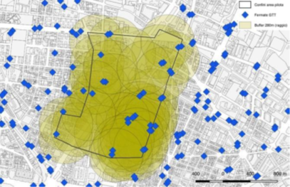
Source: Geoportale web platform, Adapted from (CESBA MED n.d.).
The accessibility of the public transportation network is estimated using the GIS map and the information described in step 3 of the assessment method. A buffer area is centered aroud each public transport stop using a 500 m radius, which is then combined with the data on the population served by the bus stop, avoiding double counting in case of buffer overlaps. The process is visualized in Figure 31. The public transportation stops are identified by the blue squares, all with public transit running at least every 20 min during peak periods. The proximity buffers of the transit stops are identified by yellow circles in Figure 31. Accordingly, the NI submetric was derived as 672 892 inhabitants that live within 0.5 km public transit running at least every 20 min during peak periods. The criteria is not satisfied for a small percentage of inhabitants living in the area outskirts of the urban scale project.
- Population sub-metric evaluation: the total number of inhabitants in the area of the urban scale project is reported at 723 540.
S.4.5 score evaluation: the metric score estimated as the ratio of NI (quantified in step 1) to P (quantified in step 2), leading to the number of inhabitants within the area of the urban scale project that live within 0.5 km public transit running at least every 20 min during peak periods, is compared against the score of the baseline metric (Tbaseline) at local level. Having evaluated the NI and P sub-metric scores and setting the local baseline metric score at the average European value of 90 %, S.4.5 score is evaluated using Equation (65), as follows (Equation (75)).
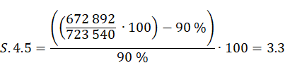
(75)
Having evaluated the scores of S.4.1, S.4.2, S.4.3, S.4.4, and S.4.5 indicators, the S.4 score is evaluated by using Equation (57), considering the indicator weights related to the combination of the project classification as renovation/residential. S.4 results into a score equal to 39.5 that corresponds to the Acceptable performance class (Figure 26, renovation/residential), as reported in Table 31.
Table 31. Example of S.4 evaluation (neighbourhood/urban scale).
| Indicator | S.4.1 | S.4.2 | S.4.3 | S.4.4 | S.4.5 |
| Indicator score | 78.9 | 11.5 | 88.7 | 16.5 | 3.3 |
| S.4 score | 0.25 • 78.9 + 0.15 • 11.5 + 0.15 • 88.7 + 0.25 • 16.5 + 0.2 • 3.3 = 39.5 | ||||
| S.4 performance class | Acceptable | ||||
| S.4 performance class score (PCSS.4) | 45 | ||||
Source: JRC.
The S.4 KPI can attain a performance class higher than Acceptable by considering a group of improvements. First, an increase of the number of EV‑recharging stations in the public parking facilities by 50 %, corresponding to a new total number of 83 EV‑recharging stations, can be considered, thus improving the S.4.1 indicator. Expanding the length of bicycle paths and lanes in the urban area with a width not less than 1.5 m at 212 km, leads to the improvement of S.4.2 indicator. In addition, efforts will focus on improving the public transport services focusing on S.4.4 and S.4.5 indicators. Accordingly, the NPTT is improved by 35 % to reach a total of 137.7 million annual number of trips operating within the area of the urban scale project. The number of public transportation stops running at least every 20 min during peak periods to cover the entire population, thus the NI sub-metric will cover the entire population.
Based on the improved scenario above, the new score of S.4.1 indicator is estimated according to Equation (76), indicating that the new number of EV-recharging stations exceeds the baseline score, so the indicator score is set equal to 100 corresponding to the maximum score possible.
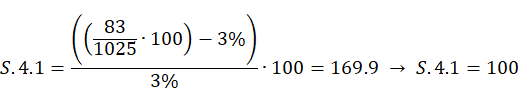
(76)
The new score of S.4.2 indicator is estimated according to Equation (77), indicating that the expanded length of bicycle paths and lanes in the urban area leads to a new indicator score equal to 95.3.
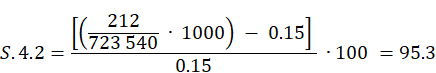
(77)
The new score of S.4.4 indicator is estimated according to Equation (78), indicating that the improved public transport services will increase the number of trips operating within the area of the urban scale project, so the new indicator score becomes 57.3.
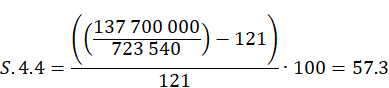
(78)
The new score of S.4.5 indicator is estimated according to Equation (79), indicating that with the improved public transport services all the inhabitants within the area of the urban scale project will have access to public transit within 0.5 km running at least every 20 min during peak periods, so the indicator score is set equal to 11.1 corresponding to the maximum score possible.
(79)
Based on the new scores of S.4.1, S.4.2, S.4.4 and S.4.5 indicators, S.4 results into a new score estimated equal to 69.1 that corresponds to the Acceptable performance class (Figure 30, renovation/residential), as reported in Error! Reference source not found..
Table 32. Example of S.4 evaluation (neighbourhood/urban scale) following the improvement of S.4.1 score.
| Indicator | S.4.1 | S.4.2 | S.4.3 | S.4.4 | S.4.5 |
| Indicator score | 100 | 95.3 | 88.7 | 57.3 | 11.1 |
| S.4 score | 0.25 • 100 + 0.15 • 95.3 + 0.15 • 88.7 + 0.25 • 57.3 + 0.2 • 11.1 = 69.1 | ||||
| S.4 performance class | Acceptable | ||||
| S.4 performance class score (PCSS.4) | 45 | ||||
Source: JRC.
3.8 Minimise non-energy related environmental impacts to air and water (S.5)
3.8.1 Description and assessment
At building scale, minimise non-energy related environmental impacts to air and water (S.5) KPI is assessed through the following two indicators:
— Indoor air quality (S.5.1).
— Water consumption (S.5.2).
S.5 score is evaluated according to Equation (80) using the same indicator weights (wS.5.j) for all the different combinations of the project classification according to type (i.e. newbuild/renovation)/main use (i.e. residential/non-residential) of a building scale project, as reported in Table 5.
(80)
S.5 KPI thresholds to associate the KPI score to the corresponding KPI performance class at building scale are illustrated in Figure 32.
Figure 32. S.5 performance classes and thresholds (building scale).

Source: JRC.
At neighbourhood/urban scale, minimise non-energy related environmental impacts to air and water (S.5) is assessed through one indicator, as follows:
— Ground water recharge: permeability (S.5.2), through ground permeability.
The S.5.1 indicator, considered at building scale, is not applicable for neighbourhood/urban scale projects. Accordingly, S.5.1 is omitted in the evaluation of the S.5 score at neighbourhood/urban scale according to Equation (81) using the same indicator weights (wS.5.j) for all the different combinations of the project classification according to type (i.e. newbuild or renovation)/main use (i.e. residential or residential/non-residential) of a neighbourhood/urban scale project, as reported in Table 5.
(81)
The S.5 thresholds to associate the KPI score to the corresponding KPI performance class at neighbourhood/urban scale are illustrated in Figure 33.
Figure 33. S.5 performance classes and thresholds (neighbourhood/urban scale).

Source: JRC.
3.8.2 Indoor air quality (S.5.1)
The indoor air quality (S.5.1) indicator is considered exclusively at building scale. Indoor air pollution sources originate from human activities and indoor sources, such as cleaning or fuel combustion for cooking and heating, and even emissions from furniture and construction materials. Building ventilation can control and improve indoor air quality; however the prevailing outdoor conditions have a direct impact on the building performance in relation to the energy use for mechanical ventilation and play a determinant role in naturally ventilated buildings.
The S.5.1 indicator is evaluated based on Level(s) indicator 4.1 ‘Indoor Air Quality’ (Dodd et al. 2021a, c), in accordance with the European standard EN 16798-1 (CEN, 2019). The S.5.1indicator considers air pollutants like volatile organic compounds (VOCs) emitted from materials, formaldehyde and carbon dioxide (CO2). The indicator assesses the concentration levels of air pollutants for a healthy indoor environment of a building scale project and provides an approach for ensuring suitable IAQ for occupants by recording the future sources of pollutants (e.g. intakes of outdoor air, etc.) or reducing the concentration levels with different ventilation strategies. The S.5.1 indicator assesses the reduction of annual concentration of each one of the above mentioned pollutants against a baseline concentration level, which is the limit value of each pollutant, for the protection of human health.
S.5.1 score, which ranges between 0 and 100, is evaluated according to a four-step framework that consecutively estimates the scores of specific sub-metrics and metrics to finally evaluate the indicator score, as follows:
Identification of concentration limits of indoor CO2: in modern buildings, an increase in CO2 above typical background air concentrations of 350-500 particles per million (ppm) in building spaces will be due to human respiration (Dodd et al., 2021c). Although a high CO2 level itself can cause human sensory discomfort (e.g. at levels of several thousand ppm), it is unlikely that concentrations in indoor air would reach such high levels. Projected CO2 levels can be used to design ventilation systems and in-situ monitoring of CO2 in specific building zones can be used as a feedback signal to control ventilation rates for those same zones (e.g. in meeting rooms where CO2 levels could vary significantly).
Possible sources of VOC emissions include building construction products and materials like ceiling tiles, paints and varnishes, textile floor and wall coverings, laminate and flexible floor coverings, wooden floor coverings, associated adhesives and sealants.
Air pollutant concentration levels (Cpollutant) for building categories metric evaluation: the air pollutant concentrations can be estimated for newbuild projects and/or measured in the indoor air for renovation projects of existing buildings, as follows:
a) Newbuild projects, simulations can be used to predict VOC concentrations in buildings. Estimations can be performed with (i) non-physical empirical (statistical) models derived from measurement, such as Markov process models, and autoregressive moving average models, and/or (ii) physical models that are more accurate (Huang and Haghighat, 2003). However, physical models require data on material VOC emission properties which may not always be available. The US Environmental Protection Agency (EPA Air Quality Modeling n.d.), has made available user-friendly programs that can be used to perform indoor air quality modelling.
b) Renovation projects of existing buildings, measurements can be performed using VOC analyzers, according to ISO 16000-6 (ISO, 2021) following the general guidelines of sampling strategies of ISO 16000-1 (ISO, 2004). Measurement procedures for formaldeyde are performed according to the active sampling method of ISO 16000-3 (ISO, 2022) or the diffusing sampling method of ISO 16000-4 (ISO, 2011) that is suitable for measurements in atmospheres with conventional indoor air, relative humidity and for monitoring at air velocities as low as 0.02 m/s.
The baseline metric score and design concentration levels of air polluntants depend on the building type and the expectations level of indoor air quality in a building space. According to EN 16798‑1 (CEN, 2019), there are four categories of expected indoor environmental quality (i.e. category-I, category-II, category-III, and category-IV), characterised by specific levels of air pollutant concentration. Category-I is the highest level of expectation, also recommended for spaces occupied by very sensitive and fragile persons with special requirements like some disabilities, sick, very young children and elderly persons, to increase accessibility. Category-II is the normal level of expectation, Category-III is the acceptable, moderate level of expectations, and Category-IV is the lowest level of expectation, acceptable only for a limted part of the year. Higher expectations are related to better control of IAQ and lower levels of concentration of air pollutants, but also generally to higher energy consumption.
For existing buildings, in-situ periodic monitoring of particulate emissions during high occupancy periods can provide the necessary data for assessing the indoor conditions.
Ventilation rate (qtot) evaluation: two main approaches can be considered to estimate the ventilation rates, namely (i) default ventilation rates, and (ii) perceived air quality.
The first approach based on the default ventilation airflow rates for the four IAQ categories (I, II, III, and IV) is the simpliest method to estimate the ventilation rate, according to Level(s) indicator 4.1 Indoor Air Quality (Dodd et al. 2021a, c). The default ventilation rates for a room in an office building range from 5.5 (category-IV) to 20 (category-I) l/s/person and from 0.55 (category-IV) to 2 (category-I) l/s/m2. When applied to a specific building zone (in terms of occupancy density), the default ventilation rates are estimated for a desirable category. The default predefined ventilation airflow rates, according to EN 16798-1 (CEN, 2019), are expressed by the total design ventilation for people and building components (qtot); design ventilation per unit floor area (q/m2), design ventilation per person (qp); design air change rates per hour (ACH); design opening areas (Atot). The supply air flow per person range from 4 (category-III) to 10 (category-I) l/s/person, the supply air flow based on perceived IAQ for adapted persons from 1.5 (category-III) to 3.5 (category-I) l/s/person or per unit floor area from 0.1 (category-III) to 0.25 (category-I) l/(s.m2) (CEN 2019). Finaly, the total ventilation including air infiltration range from rom 0.35 (category-III) to 0.49 (category-I) l/(s.m2) or from 0.5 to 0.7 ACH, respectively (CEN 2019). Category IV is intended for the evaluation of IAQ in existing buildings where the space for installations is limited and the total ventilation including air infiltration is 0.23 l/(s.m2) or 0.4 ACH.
For non-residential buildings, during unoccupied periods when the ventilation system is shut off, the minimum amount of air to be delivered prior to occupancy is 0.5 ACH of the zone to be ventilated. In case the ventilation rate is lower, the total air flow rate for diluting emissions from building is between 0.15 and 0.6 l/s.m2 of floor area.
For residential buildings, the total air flow rate for dealing with building materials emissions is between 0.1 and 0.15 l/s.m2 of floor area.
The second assessment approach based on the perceived air quality focuses on the capability of the ventilation system to remove emissions from people (bio-effluents) and from the building. Specifically, reference ventilation rates (expressed in l/s/person) account for the removal/dilution of bio-effluents to different IAQ categories (and expected occupant dissatisfaction rates), and reference ventilation rates (expressed in l/s/m2) account for the removal/dilution of emissions from the building to different IAQ categories and type of buildings, differentiated in very low, low, and non-low polluting building, according to EN 16798-1 (CEN, 2019).
A low polluting building means that the majority of the materials are low polluting. Examples of low polluting materials are natural traditional materials (e.g. stone and glass), which are known to be safe with respect to air pollutant emissions. In addition, materials have emissions of total volatile organic compounds (TVOC) below 0.2 mg/m²h, formaldehyde below 0.05 mg/m²h, ammonia below 0.03 mg/m²h, carcinogenic compounds (IARC) below 0.005 mg/m²h and are not odorous (dissatisfaction with the odour is below 10%).A building is very low polluting if all materials are very low polluting and indoor smoking has never been allowed. Very low polluting materials are natural traditional materials (e.g. stone, glass and metals). In addition, materials have emissions of TVOC below 0.1 mg/m²h, formaldehyde below 0.02 mg/m²h, ammonia below 0.01 mg/m²h, IARC below 0.002 mg/m²h, and dissatisfaction with the odour is below 10%.
The total ventilation rate for the breathing zone is assessed according to Equation (82), which combines the ventilation to handle emissions from people and building materials for the different categories. Specifically, in equation (82), data for qp that is the ventilation rate for occupancy per person (expressed in l/s.person) and qBthat is ventilation rate for emissions from building materials (expressed in l/s.m2) can be retrieved from EN 16798-1 (CEN, 2019).
(82)
where qtot = total ventilation rate for the breathing zone, l/s; n = design value for the number of the persons in the room; qp = ventilation rate for occupancy per person, l/(s.person); Au = useful internal floor area, m2; qB = ventilation rate for emissions from building materials, l/(s.m2).
The design ventilation rates for non-adapted persons for diluting emissions (bioeffluents) from people range from 2.5 (category-IV) to 10 (category-I) l/s/person, with an expected percentage of dissatisfied people at 40 % (category-IV) to 15 % (category-I) (CEN 2019). The design ventilation rates for diluting emissions from different type of buildings range for very low polluting buildings from 0.15 (category-IV) to 0.5 (category-I) l/(s.m2); for low polluting buildings from 0.3 (category-IV) to 1.0 (category-I) l/(s.m2); and for non low-polluting buildings from 0.6(category-IV) to 2.0 (category-I) l/(s.m2). In all cases, the minimum total ventilation rate for health is 4 l/s/person (CEN 2019).
- S.5.1 score evaluation: The S.5.1 score is evaluated according to Equation (83) as a ratio, in which the numerator is the difference of the score of a baseline metric (Tbaseline), corresponding to the maximum concentration level of the examined air pollutant, against the Cpollutant metric (i.e. estimated/measured concentration level of an air pollutant, e.g. VOC, Formaldehyde, CO2, as evaluated in step 2) and the denominator is the score of the same baseline metric. The ratio is multiplied by 100, so that the indicator score can be expressed as a dimensionless value that varies between 0 and 100.
 |
(83)
where Cpollutant= concentration level(simulated or/and measured accordingly for new or existing buildings) of the air pollutant (e.g., VOC, Formaldehyde, CO2) in (μg/m3 or ppb according to air pollutant), Tbaseline= emission limit value of the examined air pollutant (e.g., VOC, Formaldehyde, CO2) in (μg/m3 or parts per billion (ppb) according to air pollutant).
If the Cpollutant metric score is lower than the score of the baseline metric, S.5.1 results into a positive score, noting though that the indicator maximum score cannot exceed 100. If the Cpollutant metric score exceeds the baseline metric score, leading the difference in the numerator to be negative, S.5.1 results into a negative score indicating that the performance achieved does not satisfy the baseline metric and the indicator score is set to zero (0). For new buildings, the indoor air quality should at least meet the minimum requirements. For existing buildings may consider using as a baseline the average reported emissions value and track the relatively lower emissions and improvements.
The score of the baseline metric depends on the air pollutant considered and relevant data on the maximum concentration level of a specific air pollutant can be retrieved from the following available standards and/or resources: (i) Standard 62.1-2022 on ventilation and acceptable indoor air quality (ASHRAE, 2022), (ii) OSHA - Occupational Safety and Health Administration, Carbon Dioxide Exposure Limits (OSHA n.d.), and (iii) WELL Building Standard; Total volatile organic compounds (TVOC) less than 500 μg/m³; Formaldehyde: 27ppb (WELL n.d.). A typical score for the baseline metric score for acceptable indoor air quality that is often used for CO2 concentrations is 1000 ppm (Felgueiras et al., 2023), although several other indoor environmental factors (e.g. temperature, humidity, particulate matter concentrations) and other relevant factors (e.g. occupancy, activity, length of time a space has been occupied) influence IAQ and ventilation system performance (Persily 2022). Values far above the expected baseline may indicate that the ventilation is not sufficient and result to poor indoor air quality.
3.8.3 Water consumption (building scale) or ground water recharge: permeability (neighbourhood/urban scale) (S.5.2)
At building scale, the water consumption (S.5.2) indicator is evaluated based on Level(s) indicator 3.1 ‘Use stage water consumption’ (Donatello et al. 2021a), which promotes efficient use of water resources and use of wastewater (grey water, rainwater). It is worth noting that the total water consumption of a building scale project for the evaluation of S.5.2 indicator includes the water consumed in sanitary fittings/devices and the water‑using appliances, also considering greywater (i.e. wastewater from sinks, wash basins, showers, baths, washing machines and dishwashers, excluding wastewater from WCs and urinals) and rainwater (i.e. rainwater collected from roofs, and/or from other impermeable or pervious ground surfaces depending on the risk of contamination and the intended end use). The use of water efficient fixtures can reduce water consumption. The reuse of greywater and rainwater can provide additional savings, and it can be applied to all building types, regardless of climate and morphology. However, the reuse of greywater mandates several complex and costly systems which occupy building space to filter and pump the water and need separate collection and distribution networks and measuring devices.
The S.5.2 score, which ranges between 0 and 100, is assessed according to a three-step framework that consecutively estimates the scores of specific sub-metrics and metrics to finally evaluate the indicator score, as follows:
- Water‑using appliances, sanitary devices and fittings identification: all the water‑consuming appliances and sanitary devices used in a building scale project need to be identified along with details that influence the water consumption (e.g. toilet flush volumes, maximum flow rates for taps, size of irrigated areas, etc.). Furthermore, any architecturally significant building features that relate to water consumption (e.g. gardens, green roofs, green walls, etc.) shall also be accounted for.
Data collection on water consumption: relevant data to obtain the water consumption of a building scale project may be derived from different sources depending on renovation or newbuild projects, as follows:
a) Renovation projects, water consumption is obtained from measured data including meter readings of potable water consumption (e.g. from the water utility) and, potentially, meter readings of supplied rainwater and/or greywater. Alternatively, relevant data include: (i) estimated building occupancy rate (average full time equivalent occupants in the building per day), (ii) estimated number of days that the building is occupied for normal use (e.g. offices week work schedule and national holidays, exclude residents’ holiday days), and (iii) estimated number of visitors, if they are significant compared to the building permanent occupants (mostly for non-residential buildings). When assessing visitors, it should also be considered against full time equivalents (e.g. 4 visitors staying for 2 hours could be equivalent to 1 person working 8 hours).
b) Newbuild projects, water consumption of a new building is estimated using default occupancy rates (e.g. EN 16798-1:2019 (ANNEX A8), ISO 52000-1:2017 (ISO, 2017a)) and default values for water consumption rates for all sanitary fittings/devices and water-using appliances, as summarised in Table 33. Daily uses are expressed per occupant, e.g. flushes per occupant per day.
Table 33. Water consumption default data for water-using appliances and sanitary devices/fittings.
| Building use factor | 335 | days/annum | ||
| Sanitary devices | Consumption rates | Usage factor (per occupant, per day) | ||
| Toilet (full flush) | 7.5 | L/full flush | 1 | flushes/o/day |
| Toilet (small flush) | 4.5 | L/small-flush | 4 | flushes/o/day |
| Bathroom tap | 10 | L/minute | 75 | seconds/o/day |
| Shower | 12 | L/minute | 360 | seconds/o/day |
| Bath-tub | 185 | L/bath | 0.11 | baths/o/day |
| Kitchen tap | 12 | L/minute | 240 | seconds/o/day |
| Sanitary devices sub-total | ||||
| Water using appliances | Consumption rates | Usage factor | ||
| Dishwasher | 11.5 | L/cycle | 0.4 | cycles/o/day |
| Washing machine | 43.5 | L/cycle | 0.3 | cycles/o/day |
| Appliances sub-total | ||||
| Irrigation | 108.7 | L/d | ||
Source: Donatello et al., 2021a.
The demand for irrigation depends on the type of vegetation (e.g. trees, bushes, creeping plants, mixed plants, or lawn grass), the water demand category for the species planted, the microclimate and the vegetation density.
- Potable water consumption (PWC) metric evaluation: the PWC metric is the daily potable water consumption in litres per occupant, simulated or measured depending on newbuild or renovation projects, (expressed as Litres/occupant/day) that is estimated as the result of the total water consumption from all sanitary devices and water-using appliances of a building project minus the non-potable (greywater and rainwater) water consumption, normalised by the number of occupants.
- S.5.2 score evaluation: the S.2.1 score is estimated according to Equation (84) as a ratio, in which the numerator is the difference of the score of a baseline metric (Tbaseline), corresponding to the average national (or regional) daily water consumption per occupant (expressed in L/occupant/day), against the PWC metric (evaluated in step 3), and the denominator is the score of the same baseline metric, multiplied by 100, so that the indicator score can be expressed as a dimensionless value that varies between 0 and 100.
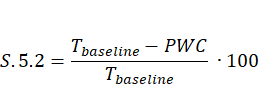 |
(84)
If the PWC metric score is lower than the score of Tbaseline metric, S.5.2 results into a positive score, noting though that the indicator maximum score cannot exceed 100. If the PWC metric score exceeds the baseline metric score, leading the difference in the numerator to be negative, S.5.2 results into a negative score indicating that the performance achieved does not satisfy the baseline metrict and the indicator score is set to zero (0). The water consumption should at least meet the minimum requirements for new buildings that have installed new fittings that are water efficient. For existing buildings to be renovated it may consider using as a baseline metric the average water use and track the relatively lower water consumption and improvements.
The score of the baseline metric to be used in Equation (84) can be set for residential builings at national level by considering the national averages for annual households' water use from public supply (expressed in m3/inhabitant), available from Eurostat (2023a). Similarly, the score of the baseline metric can be set at EU level, by considering the median value of the aforementioned national data, that is estimated equal to around 40-50 m3 per inhabitant per year, equivalent to 109 to 137 litres per day per inhabitant. National data of each EU Member State directly expressed as averages daily water consumption per occupant for residential buildings are also available for 2021 (EurEar, 2021). For non-residential buildings, there are significant variations of water consumption depending on the building use (e.g. office, school, hotel), occupancy, equipment, operations, and landscape area. Metrics that are specific to the building use may better reflect the different activities and water consumption benchmarks. For example, functional metrics (e.g. water consumption per guest-night in a hotel, per patient in a hospital, per meal served in a restaurant), people metrics (e.g. water use per employee in an office building or per student in a school) and physical characteristics of the facility (e.g., water use per unit floor area) that is the most widely reported metric (EPA, 2024). Typical water use data may be difficult to find for non-residential buildings at local or national level. In the absence of local data, a good starting point is to use average values for the normalized water use intensity as water consumption per unit floor area per year for similar building uses (EPA, 2024). For example, 590.0 litres per m2 per year for an office (or 22788.2 litres per employee per year), 441.7 litres per m2 per year for a school (or 42396.6 litres per student per year), 2119.6 litres per m2 per year for a hotel (or 126811.3 litres per guest room per year), and 2269.9 litres per m2 per year for a hospital (or 405039.1 litres per hospital bed per year). It is also possible to use water consumption records over a period of a few years, if available, to derive an average score of the baseline metric for a specific building. In all cases, shall use the same water consumption metric PWC and baseline in Equation (84) to calculate S.5.2.
At neighbourhood/urban scale, the ground water recharge: permeability (S.5.2) indicator is considered as relevant issues relate to the capacity of the soil to transmit water. Soil sealing by covering of soil surfaces with materials, such as concrete and asphalt, for new buildings, roads, parking places, as well as other public and private spaces, reduces ground permeability and its capacity to transmit water to the soil. This limits the water recharging of aquifers and reduces effluents, while often increasing the risk of flooding and water scarcity, also contributing to global warming.
S.5.2 score, which ranges between 0 and 100, is evaluated according to a four-step framework that consecutively estimates the scores of specific sub-metrics and metrics to finally evaluate the indicator score, as follows:
Data collection: data on (i) soil characteristics and (ii) surface of developed (i.e. occupied by constructions) and/or undeveloped areas (i.e. areas uncovered by structures but with different paving) need to be collected, as follows :
a) Soil characteristics: each type of soil/ground cover land use is characterised by a weighting factor related to its potential for vegetation growth and nature implementation, e.g. sealed surface = 0; semi-open surfaces = 0.2; surfaces with vegetation, connected to soil below = 1 (City of Berlin, 2020a).
b) Surface of developed (Sa,1) and undeveloped (Sa,2) areas within the designated urban area need to be estimated, thus including areas with a different paving or occupied by constructions (i.e. green areas, surfaces paved with asphalt, surfaces occupied by buildings, etc.)
Degree of built area (DBA) sub-metric evaluation: the total surface of a designated urban area (Sa), expessed in m2, is estimated as the sum of the surface of the developed areas (Sa,1) (i.e. areas covered with structures) within the designated urban area and the surface of the undeveloped areas (Sa,2) (i.e. areas uncovered by structures) within the designated urban area. Based on this data, the degree of built area (DBA) is estimated as the ratio of the surface of the developed areas to the total surface of the designated urban area, according to Equation (85).

(85)
It is worth noting that the DBA sub-metric score is used to estimate the score of the baseline metric (Tbaseline) the of the needed soil permeability of the designated urban area, within the step 4 of the framework for the evaluation of S.5.2 score.
Real permeability of the soil (Sa,perm)sub-metric evaluation: different surface types are characterised by a corresponding different real permeability of the soil depending on specific pearmibility weighting factors. Hence, the real permeability of the soil of the designated urban area (Sa,perm) sub-metric, expressed in m2, is estimated as the sum of the products of the i-th different surface type within the designated urban area (Sa,i), expressed in m2, by the corresponding permeability weighting factors (αi) per unit surface, according to Equation (86). Specifically the permeability weighting factors for each different i-th surface type (αi) are reported in Table 34.
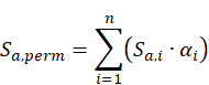
(86)
Table 34. Different surface types and corresponding permeability weighting factor per unit surface.
| Surface type (Sa,i) | Weighting factor (ai) | Description of surface type |
| Sealed surfaces (impermeable surface) | 0.0 per m² | Surface is impermeable to air and water and has no plant growth (e.g., concrete, asphalt, slabs with a solid subbase). |
| Partially sealed surfaces (semi-impermeable surface) | 0.1 per m² | Surface is permeable to water and air; as a rule, no plant growth (e.g., clinker brick, mosaic paving, slabs with a sand or gravel subbase). |
| Semi-open surfaces | 0.2 per m² | Surface is permeable to water and air, water infiltration, but no plant growth (e.g., sand, gravel, clinker brick with high water infiltration). |
| Green surfaces | 0.4 per m² | Surface is permeable to water and air, water infiltration and plant growth (e.g., gravel with grass, wooden cobbles, grass paving blocks). |
| Surfaces with vegetation, connected to the soil below | 1.0 per m² | Vegetation connected to soil below, available for development of flora and fauna. |
| Rainwater infiltration per m² of roof area | 0.2 per m² | Rainwater infiltration for replenishment of groundwater; infiltration over surfaces with existing vegetation. |
| Water surface | 0.5 per m² | Rainwater fed water surface. |
| Surfaces with vegetation, unconnected to the soil below, small substrate thickness | 0.5 per m² | Surfaces with vegetation that have no connection to the ground and 20 to 40 cm of soil covering. |
| Surfaces with vegetation, unconnected to the soil below, medium substrate thickness | 0.6 per m² | Surfaces with vegetation that have no connection to the ground and 41 to 80 cm of soil covering. |
| Surfaces with vegetation, unconnected to the soil below, large substrate thickness | 0.7 per m² | Surfaces with vegetation that have no connection to the ground and 81 to 150 cm of soil covering. |
| Surfaces with vegetation, unconnected to the soil below, very large substrate thickness | 0.9 per m² | Surfaces with vegetation that have no connection to the ground but more than 150 cm of soil covering. |
| Vertical greenery with connection to the ground | 0.5 per m² | Direct connection of the vertical greenery with the soil, supply with nutrients and water directly over the roots in the soil. |
| Vertical greenery without connection to the ground | 0.7 per m² | Vertical or horizontal vegetation on a wall without direct connection to the soil on the ground, permanent planters supplying the vegetation, with artificial irrigation. |
| Extensive roof greening | 0.5 per m² | Nature-like design of the roof surfaces with a substrate thickness under 20 cm without artificial irrigation. Through systems for water retention the metric can be increased to 0.6 (only for extensive roof greening). |
| Semi-intensive roof greening | 0.7 per m² | Mixture of extensive and intensive roof greening with a substrate thickness of 15 to 50 cm (depending on the chosen plant), usually in combination with artificial irrigation. |
| Intensive roof greening | 0.8 per m² | Design of the roof similar to ground-based green areas with a substrate thickness more than 50 cm, usually in combination with artificial irrigation. |
Source: City of Berlin, 2020a
4. S.5.2 score evaluation:
The metric concerning the real permeability of soil of the designated urban area over the total surface of the deisgnated urban area is estimated as the ratio of Sa,perm (quantified in step 3) to the total surface (Sa), expressed as a percentage. Subsequently, the S.5.2 score is assessed according to Equation (87), as a ratio in which the numerator is the difference of the aforementioned metric score against the score of a baseline metric (Tbaseline) of the needed permeability of soil , and the denominator is the score of the same baseline metric, multiplied by 100, so that the indicator score varies between 0 and 100.
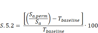 |
(87)
If the metric score of the share of the real permeability soil over the total surface area is greater than the baseline metric score, S.5.2 results into a positive score, noting though that the indicator maximum score is 100. A higher score implies that the area is more permeable, and a lower score indicates that the area is less permeable. If the metric score of the share of the real permeability soil over the total surface area is lower than the score of the baseline metric, leading to a negative difference in the numerator, S.5.2 score points out that the indicator performance does not satisfy the baseline metric and the and the indicator score is set to zero (0). For newbuild project, the normalised permeability should at least meet the minimum requirements. For the assessment of renovation projects of existing projects it is possible to use as a baseline metric score the current status and track the relative improvements.
The score of the baseline metric (Tbaseline) of the needed permeability in Equation (87) can be estimated according to the different types of land use, the existing degree of built area, and project type of development (alterations or extensions due to renovation projects, or newbuild projects), as summarised in Table 35.
Table 35 Baseline metric score of the needed soil permeability according to land use, degree of build area and project development type.
| Renovation project (existing buildings) | Newbuild project | |||
| Degree of built area (DBA) sub-metric score | Baseline metric score (ratio) | Baseline metric score (%) | Baseline metric score (ratio) | Baseline metric score (%) |
| Residential units (Residential use only and mixed use with no commercial use of open space) | ||||
| up to 0.37 | 0.60 | 60 | 0.60 | 60 |
| 0.38 to 0.49 | 0.45 | 45 | ||
| over 0.50 | 0.30 | 30 | ||
| Commercial use (Commercial use only and mixed use with commercial use of open space) | ||||
| 0.30 | 30 | 0.30 | 30 | |
| Public facilities (for cultural or social purposes) | ||||
| up to 0.37 | 0.60 | 60 | 0.60 | 60 |
| 0.38 to 0.49 | 0.45 | 45 | ||
| over 0.50 | 0.30 | 30 | ||
| Schools (general-education schools, vocational centres, education complexes, outdoor sports facilities) | ||||
| 0.30 | 30 | 0.30 | 30 | |
| Nursery schools and day care centres | ||||
| up to 0.29 | 0.60 | 60 | 0.60 | 60 |
| 0.30 to 0.49 | 0.45 | 45 | ||
| over 0.50 | 0.30 | 30 | ||
| Technical infrastructure | ||||
| 0.30 | 30 | 0.30 | 30 | |
Source: City of Berlin, 2020b.
3.8.4 Example (S.5)
The example for the evaluation of the S.5 KPI is carried out by considering two projects referring to a building and an urban scale project, respectively.
The building scale project refers to a residential multifamily building, located in Greece, with a useful internal floor area of 2700 m2 and an occupancy estimated equal to 88 people. The desirable indoor air quality corresponds to the category-III for a building with acceptable, moderate level of expectations of indoor air quality. A typical dwelling with representative sanitary devices and water‑using appliances can be considered within the building to estimate the water consumption and consequently extrapolate for the entire building. Garden irrigation can also be accounted with a typical water use profile. Each typical dwelling is also equipped with a small rainwater collector of 20 m2 surface area, which can cover the needs for irrigation purposes.
The evaluation of the S.5 KPI at building scale to minimise the building non-energy environmental impacts to indoor air and water by assessing the ventilation rates for acceptable indoor air quality (S.5.1) and the freshwater consumption (S.5.2).
The S.5.1 score is evaluated according to the three-step framework, as reported in Section 3.8.2, leading to the estimation of the scores of the sub-metrics and metrics to finally evaluate the indicator score, as follows:
- Identification of concentration limits of indoor CO2: the concentration of CO2 emissions are considered to characterise the indoor air quality of the spaces of the building scale project. The IAQ category and expectation levels for the building scale project refer to the category-III, for an acceptable, moderate level of expectation.
- Air pollutant concentration levels (Cpollutant) for building categories metric evaluation: the CO2 concentration was estimated as mean value at 1800 ppm.
- Ventilation rate (qtot) evaluation: since the IAQ category and expectation levels for the building scale project refer to the category-III, for an acceptable, moderate level of expectation, the ventilation rate for occupancy per person (qp) is 0.4 l/s/person and the ventilation rate for emissions from building materials (qB) is 0.8 l/(s.m2) for a non-low polluting building, according to EN 16798-1 (CEN, 2019). The total ventilation rate (qtot) for the breathing zone is evaluated by using Equation (88) to combine the ventilation to handle emissions from people and the building materials in the space for a non-low polluting building, as follows (Equation (88)):
 |
(88)
5. S.5.1 score evaluation: having evaluated the CO2 concentration metric equal to2800ppm (estimated in step 2) and considering the score of the baseline metric for the indoor CO2 equal to 1000 ppm (Felgueiras et al., 2022), the S.5.1 score is estimated using Equation (83), as follows (Equation (89)). The S.5.1 indicator results into a negative score since the indoor CO2 concentration is greater that the score of the baseline metric, thus indicating that the performance achieved is not sufficient and the indicator score is set to zero (0).
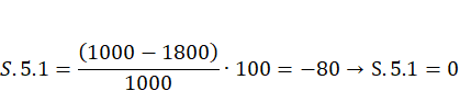 |
(89)
An effective action to improve the indoor air quality and decrease the indoor concentrations consists in increasing the ventilation rate. However, this will increase energy consumption for mechanical ventilation. Alternatively, the CO2 concentration may be reduced to a mean value below 1000 ppm, to obtain a similar improvement due to the increase of the ventilation rate.
The S.5.2 score is evaluated according to the four‑step framework, as reported in Section 3.8.3, leading to the estimation of the scores of the sub-metrics and metrics to finally evaluate the indicator score, as follows:
- Water-using appliances, sanitary devices and fittings identification: A typical dwelling within the building project is considered to identify (i) the sanitary devices, i.e. one toilet (full and small flush), one bathroom tap, one shower, one bath-tub, one kitchen tap, and (ii) water‑using appliances, i.e. one dishwasher, and one washing machine. The occupants use the building for 345 days per year (i.e. building use factor). Garden irrigation for a small, vegetated area of mixed planting with medium density, a medium water demand, with a medium microclimate, and a manual irrigation system is also considered. The typical dwelling is also equipped with a small rainwater collector of 20 m2 surface area, which can cover the needs for irrigation purposes.
- Data collection on water consumption: the water consumption of the building project is based on estimated data of consumption rates and usage factors for all the sanitary devices and water-using appiances, as reported in Figure 34, leading to a total daily water consumption per occupant equal to 199.5 litres/occupant/day.
Figure 34. Example S.5: water consumption data for sanitary devices and water‑using appliances
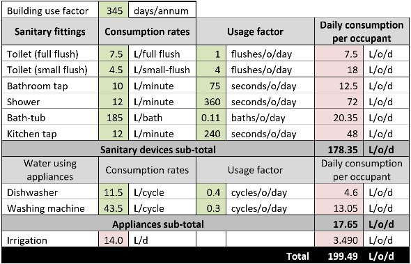
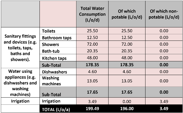
Source: Adapted from Donatello et al. 2021a
- Potable water consumption (PWC) metric evaluation: the building total water consumption is estimated equal to 199.5 L/o/d (step 2) of which 196.0 L/o/d is the potable water consumption, corresponding to the PWC metric score, while the remaining 3.5 L/o/d is the non-potable water consumption, which refers to the water used for irrigation purposes.
- S.5.2 score evaluation: having estimated the PWC metric (step 3), the S.5.2 indicator is evaluated in relation to the national, i.e. Greek, context by setting the score of the baseline metric at Greek level. Specifically, the score of the baseline metric corresponds to the average daily potable water consumption per inhabitant in Greece, which was estimated equal to 139 L/o/d in 2021 (EurEau, 2021). Accordingly, the S.5.2 score is estimated using Equation (84), as follows (Equation (90)). The indicator is negative, as the daily potable water consumption of the building scale project exceeds the average consumption of the residential buildings in Greece. Hence, the S.5.2 score is set equal to zero (0).
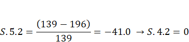 |
(90)
Having evaluated the scores of S.5.1 and S.5.2 indicators, S.5 is estimated by using Equation (80) and considering the indicator weights corresponding to the project classification according to the combination of scale/type/use as building/newbuild/residential (Table 5). However, both indicators resulted into a score equal to zero (0), as they do not meet the minimum baseline metric score, thus S.5 score also equals 0 that corresponds to the Low performance class (Figure 32, newbuild/residential), as reported in Table 36.
Table 36. Example of S.5 evaluation (building scale)
| Indicator | S.5.1 | S.5.2 |
| Indicator score | 0 | 0 |
| S.5 score | 0.7 • 0 + 0.3 • 0 = 0 | |
| S.5 performance class | Low | |
| S.5 performance class score (PCSS.5) | 25 | |
Source: JRC.
It is recommended that S.5 indicator attains at least the Acceptable performance class. In this context, a scenario of improvement relying on the enhancement of both S.5.1 and S.5.2 indicators is considered.
Regarding the S.5.1 indicator, a scenario for which the examined pollutant decreases to 850 ppm is envisaged, thus the S.5.1 score is re-estimated by using again Equation (89), as follows (Equation (91)):
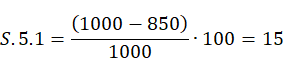
(91)
The total ventilation rate can also be re-evaluated, considering a very low polluting building, as follows (Equation (92)), leading to a significantly reduced ventilation rate that will also allow for smaller size ventilation equipment, that ensures additional energy savings for ventilation.

(92)
Regarding the S.5.2 indicator, the use of more water efficient fixtures that will reduce the total daily potable water consumption per occupant by 35 % is considered. This translates into a reduction of the daily potable water consumption per occupant to 127.4 L/o/d, that corresponds to the new score of the PWC metric. Accordingly, the S.5.2 score can be re-evaluted by using again Equation (84), as follows (Equation (93)), thus resulting into a new positive score.
 |
(93)
Based on the new scores of S.5.1 and S.5.2 indicators, S.5 results is re-estimated using again Equation (80) and resulting into a score estimated equal to 19.9 that corresponds to the Good performance class (Figure 32, newbuild/residential), as reported in Table 37.
Table 37. Example of S.5 evaluation (building scale) following the improvement of indicator scores
| Indicator | S.5.1 | S.5.2 |
| Indicator score | 15 | 8.3 |
| S.5 score | 0.7 • 15 + 0.3 • 8.3 = 13 | |
| S.5 performance class | Good | |
| S.5 performance class score (PCSS.5) | 70 | |
Source: JRC
At neighbourhood/urban scale, the project refers to an existing neighbourhood which needs to be renovated. A lot of land, that is representative for the entire neighbourhood area, is considered and it accounts for a total surface area of 500 m2, out of which 200 m2 correspond to the developed surface area, which is covered mainly with residential structures, while the undeveloped surface area, corresponding to the area not covered by buildings, is 300 m2.
The evaluation of S.5 at neighbourhood/urban scale to minimise the non-energy environmental impacts related to water resources depends exclusively on S.5.2 score, which is estimated according to the four-step framework, as reported in Section 3.8.3, leading to the estimation of the scores of the sub-metrics and metrics to finally evaluate the indicator score, as follows:.
- Data collection: data on the surface of developed and/or undeveloped areas are collected, along with the different surface types. The entire area has a total surface area (Sa) of 500 m2. The developed area (Sa,1) is equal to 200 m2, whereas the uncovered area (Sa,2) equal to 300 m2 consists of the following different surface types (Sa,i): (i) asphalt, with a surface area of 150 m2, (ii) gravel with grass, accounting for a surface area equal to 100 m2, and (iii) open green area with vegetation, accounting for as surface area equal to 50 m2
- Degree of built area (DBA) sub-metric evaluation: having collected the data in step 1, the DBA (i.e. land-structure ratio) is estimated by using Equation (86), as follows (Equation (94)):
 |
(94)
3. Real permeability of the soil (Sa,perm) sub-metric evaluation: according to data collected in step 1 on the different surface types of the uncovered area of the designated urban area, i.e. asphalt (Sa,asphalt =150 m2), gravel with grass (Sa,gravel =100 m2), and open areas with vegetation (Sa,vegetation =50 m2), the corresponding permeability weighting factors per unit surface are identified by using data in Table 34. Specifically, the permeability weighting factors for sealed surfaces, green surfaces, and surfaces with vegetation connected to the soil were considered for the asphalt (aasphalt = 0), gravel with grass (agravel = 0.4), and areas with vegetation (avegetation = 1), respectively. Based on the above, the real permeability of the soil of the designated urban area (Sa,perm) is estimated by using Equation (86), as follows (Equation (95)):
(95)
S.5.2 score evaluation: the metric score estimated as the ratio of Sa,perm (real permeability of the soil of the designated urban area, quantified in step 3) to Sa, (i.e. the total surface of the designated urban area, collected in step 1) is compared against the score of the baseline metric (Tbaseline). Specifically, the baseline metric score is set to 45 %, according to data in Table 35, considering the following combination of land use, degree of built area, and project development type, respectively: residential and mixed uses with no commercial use of open spaces, a degree of built area into the range 0.38-0.49 since the DBA of the designated urban area averages 0.4 (as estimated in step 2) for a renovation project.
Having evaluated the Sa,perm sub-metric score, the Sa,, and the baseline metric score, S.5.2 is estimated using Equation (87), as follows (Equation (96)). The indicator score is negative, as the permeability of soil of the designated urban area is lower than the baseline metric score, which means that the area does not allow for sufficient water permeability because of the soil coverage. Hence, S.5.2 is set equal to zero (0).
(96)
Based on the indicator score, the S.5 score will result equal to zero (0), as the KPI is assessed only through the S.5.2 indicator, corresponding to a Low performance class (Figure 33, renovation/residential). The indicator score can be improved by replacing the impermeable areas with vegetation. Specifically, the asphalt surface equal to 150 m2 can be converted into green areas with vegetation, so the different surface types of the uncovered area of the designated urban area become the gravel with grass (Sa,gravel =100 m2), and open areas with vegetation (Sa,vegetation = 200 m2). Consequently, the Sa,perm sub-metric can be re-estimated by using again Equation (86), as follows (Equation (97)):
(97)
Based on the new score of the Sa,perm sub-metric, the S.5.2 indicator is estimated again, according to Equation (98), resulting into a positive score.
 |
(98)
Having evaluated the new score of S.5.2 indicator, the S.5 score is estimated by using Equation (81), considering the indicator weights corresponding to the combination of the project classification according to scale/type/use into neighbourhood/urban, renovation, and residential, respectively (Table 5). Hence, S.5 results into a score corresponding to the S.5.2 score, thus attaining the Acceptable performance class (Figure 33, renovation/residential), as reported in Table 38.
Table 38. Example of S.5 evaluation (neighbourhood/urban scale).
| Indicator | S.5.2 |
| Indicator score | 6.7 |
| S.5 score | 1 • 6.7 = 6.7 |
| S.5 performance class | Acceptable |
| S.5 performance class score (PCSS.5) | 45 |
Source: JRC
3.9 Minimise non-energy related environmental impacts from the built environment (S.6)
3.9.1 Description and assessment
Minimise non-energy related environmental impacts from the built environment (S.6) KPI is assessed through one indicator, at both building and neighbourhood/urban scale:
- Construction and demolition waste (CDW) (S.6.1).
S.6 score, ranging from 0 to 100, is calculated according to Equation (99), thus corresponding to S.6.1 score.
(99)
The S.6 thresholds adopted in the self-assessment method to associate the KPI score to the corresponding KPI performance class at building, and neighbourhood/urban scales are illustrated in Figure 35 that vary only depending on a newbuild or renovation project.
Figure 35. S.6 performance classes and thresholds

Source: JRC
3.9.2 Construction and demolition waste (S.6.1)
At building scale, S.6.1 is assessed based on Level(s) indicator 2.2 ‘Construction and demolition waste and materials’ (Donatello et al., 2021, Dodd et al., 2021a). CDW originates at sites where construction, renovation or demolition of buildings and/or other construction works takes place, thus coming in many different forms and containing material from a wide range of sources, including building materials, furnishings, insulation, concrete, and asphalt. Specifically, construction waste contains a variety of materials, typically generated during the construction process. Renovation waste can contain both construction-related materials and demolition-related materials. The European List of Wastes (Commission Decision, 2014) provides a harmonized classification of the different types of waste. Specifically, the chapter 17 of the European list of wastes allows the classification of construction and demolition waste by specific codes for individual materials that can be collected separately at a construction or demolition site. It includes waste streams (i.e. hazardous and non-hazardous; inert, organic, and inorganic) resulting from construction, renovation, and demolition activities. S.6.1 indicator estimates the share of waste potentially recovered from the waste generated at the end of life of a building and aims to promote the construction and demolition waste minimisation and an efficient waste management. A complete bill of quantities (BoQ) and bill of materials (BoM) of the building scale project, as used during the construction phase of a building (relevant information are also available in S.3.2), is useful to collect relevant data for the indicator evaluation.
The S.6.1 score, ranging from 0 to 100, is evaluated according to a four-step framework estimating relevant metric and sub-metrics to finally evaluate the indicator score, as follows:
- Generated CDW (CDWG) sub-metric evaluation: the total quantity of CDW (expressed in kg) generated at the end of the life cycle (i.e. demolition stage) of a building scale project needs to be determined. In the case of a building scale renovation project, only the construction works related to the renovated part of a building are assessed. Construction plans can be used to extract data on dimensions and quantities of materials, components or elements that can be used without or after minor processing (i.e. reused materials) in a newbuild or renovation project at building scale, or quantities of materials that require significant processing (i.e. recycling materials) to be suitable for a newbuild or renovation project at building scale.
- Recovered CDW (CWDR) sub-metric evaluation: the various streams of CDW (expressed in kg) that could be recovered at the end of the life cycle (i.e. demolition stage) of a building scale project are quantified. This estimation shall be based on the design guidelines related to the Level(s) indicator 2.4 Design for deconstruction (Dodd et al., 2021b). Specifically, the indicator 2.4 in Level(s) includes estimates for each construction material or element, considering its type and the stream in which it can be classified (i.e. reuse, recycling). This quantity is disaggregated into the different types of CDW as per the chapter 17 entries of the European List of Waste (Commission Decision, 2014).
- S.6.1 score evaluation: the metric regarding the share of CDW that can be recovered for reuse/recycling/recovery at the end of the life cycle of the building over the total CDW generated is estimated as the ratio of CDWR (quantified in step 2) to CDWG (quantified in Step 1), expressed as a percentage. Subsequently, the S.6.1 score is evaluated according to Equation (100) as a ratio, in which the numerator is the difference of the score of the aforementioned metric against the score of a baseline metric of recovery rates, and the denominator is the score of the same baseline metric, multiplied by 100, so that the indicator score can be expressed as a dimensionless value that varies between 0 and 100.
 |
(100)
The higher the ratio of the recovered material, the less waste will be generated. If the metric score is greater than the score of the baseline metric, S.6.1 results into a positive score, noting though that the indicator maximum score cannot exceed 100. If the metric score is lower than the score of the baseline metric, leading the difference in the numerator to be negative, S.6.1 results into a negative score demonstrating that the indicator performance does not satisfy the baseline metric, thus the indicator score is set to zero (0).
The score of the baseline metric (Tbaseline) to be used in Equation (100) can be set based on the rationale that the ratio of material that can be recovered from CDW should at least meet the EUminimum requirement setting a recovery rate of CDW of 70 % (by weight) for 2020, according to the Waste Framework Directive (Directive, 2008). However, the recovery rates vary significantly by Member State, therefore national data may be used to set the score of the baseline metric, mainly for projects in the EU countries which already exceed the 70 % EU recovery target. An overview of relevant national recovery rates of CDW in the EU-27 are reported in Figure 36 for the period 2010-2018 (Moschen-Schimek et al., 2023).
Figure 36. Recovery rates of CDW for EU-27 during the period 2010-2018
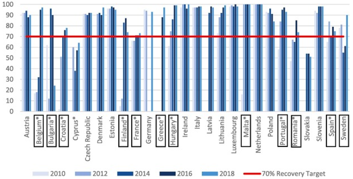
Source: Moschen-Schimek et al., 2023
At neighbourhood and urban scale, multiple building-scale assessments need to be performed by considering each building within the designated area and applying the same three-step framework defined for the evaluation of the S.6.1 score at single building scale. The evaluation of S.6.1 may also include other works for infrastructures within the designated area of the neighbourhood and urban scale project. Subsequetly, the S.6.1 score at neighbourhood and urban scale is estimated as a weighted average of the indicator scores corresponding to the separate building scale assessments.
3.9.3 Example (S.6)
The example for the evaluation of the S.6 KPI only focuses on a building scale project.
The building scale project is a new single-family house, with a useful floor area of 100 m2, which features four exterior 0.20 m‑thick concrete walls. Each wall is 10 m long and 3 m high; three out of the four walls have two windows (with the following dimensions each (1.4 m x 1.4 m), and a balcony door that is 1.4 m-long and 2.2 m-high. The fourth wall has two windows with the following dimensions each (1.4 m x 1.4 m) and a central entrance that is 1.0 m-long and 2.2 m-high featured with a timber door. Each wall is also insulated with extruded polystyrene (XPS) panels having a thichness of 0.05 m.
The evaluation of S.6 KPI at building scale to minimise the non-energy related environmental impacts of the building due to construction materials/components depends on the score of S.6.1 indiactor.
The S.6.1 score is evaluated according to the three-step framework, as reported in Section 3.9.2, leading to the estimation of the sub-metric and metric scores to finally evaluate the indicator score, as follows:
- Generated CDW (CDWG) sub-metric evaluation: the bill of materials and quantities used for the building scale project are analysed to carry out the inventory of material masses (kg) or volumes (m3), converted into the corresponding masses (kg) through the material density (kg/m3), to evaluate the total CDWG, as reported in Table 39. Specifically, the area of the exterior walls, excluding the openings and the entrance door, is equal to 92.88 m2. The wall thickness is equal to 0.2 m, so it can be inferred that a volume of materials equal to approximately 18.58 m3 has been used for the construction of the external walls. The load bearing structure of the walls corresponds to 20 % of this volume, which means approximately 3.72 m3 of concrete has been used. Additionally, the XPS insulation panels used for the walls account for a total material volume equal to 4.64 m3, considering that the insulation panels are 0.05 m thick. Finally, the entrancetimber door of the single-family house, accounts for a mass equal to around 80 kg Assuming that these building materials, i.e. concrete, XPS, and timber are the only ones being used for the building scale project, the sum of the three masses results into a total of 9135.5 kg, which corresponds to the score of the potential total CDW generated.at the end of the building lifecycle.
Table 39. Inventory of materials for the evaluation of CDWG.
| Building component | Material | Material volume (m3) | Material density (kg/m3) | Mass (kg) | |
| Wall | Total wall area1 = 92.88 m2 Thickness = 0.2 m Volume = 18.58 m3 | Concrete | 0.2 ∙ 18.58 = 3.72 | 2400 | 8916.5 |
| Wall insulation | XPS panel thickness = 0.05 m | XPS | 92.88 ∙ 0.05 = 4.64 | 40 | 139 |
| Entrance door | Timber | 80 | |||
| Potential total CDWG | 9135.5 | ||||
1 The calculation of the total area of walls excludes the area of windows and entrance door
Source: JRC.
- Recovered CDW (CWDR) sub-metric evaluation: based on the bill of materials and quantities for concrete, XPS, and timber carried out in step 1 (Table 39), it is assumed that 79 % of concrete can be recovered and 95 % of the XPS insulation will be recycled. Hence, a mass of 7044.1 kg of recovered concrete and 132.1 kg of recycled XPS insulation is obtained. Additionally, the total mass of timber used for the entrance door will be reused. The total mass of the recovered CDW at the end of the building lifecycle is obtained by summing the three partial masses of recovered concrete, recycled XPS insulation, and reused timber, resulting into a CWDR score that equals to 7256.1 kg (i.e. CWDR = 7044.1 kg + 132.1 kg + 80 kg = 7256.1 kg).
- S.6.1 score evaluation: the metric score, estimated as the ratio of CWDR (quantified in step 2) to CWDG (quantified in step 1), is compared against the score of a baseline metric (Tbaseline). Specifically, the Tbaseline score corresponds to the EU minimum requirement of the recovery rate of CDW equal to 70 %. Having evaluated the CWDR and CWDG sub-metric scores and the baseline metric score, S.6.1 score is estimated using Equation (100), as follows (Equation (101)).
 |
(101)
S.6 results into a score estimated equal to 13.5 that corresponds to the Acceptable performance class (Figure 35, newbuild/residential), as reported in Table 40.
Table 40. Example of S.6 evaluation (building scale).
| Indicator | S.4.1 |
| Indicator score | 13.5 |
| S.6 score | 1.0 • 13.5 = 13.5 |
| S.6 performance class | Acceptable |
| S.6 performance class score (PCSS.6) | 45 |
Source: JRC.
3.10 Achieve the best possible greening of the public sector in terms of its economic involvement in the sustainability of the built environment (S.7)
3.10.1 Description and assessment
Achieve the best possible greening of the public sector in terms of its economic involvement (S.7) KPI is assessed through the following three indicators:
- Social return of investment (SROI) (S.7.1).
- Degree of interdisciplinary integration (S.7.2).
- Gross value added to local economy from new business creation (S.7.3).
S.7 score, resulting into the range 0-100, is evaluated according to Equation (102).
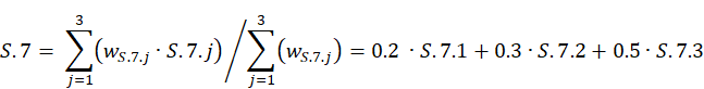
(102)
The S.7 thresholdsadopted in the self-assessment method to associate the KPI score to the corresponding KPI performance class are provided in
Figure 37. The Low, Acceptable, Good, and Excellent performance classes for the S.7 KPI correspond to the following ranges of S.7 scores, i.e. 0 ≤ S.7 < 20, 20 ≤ S.7 < 40, 40 ≤ S.7 < 80, and 80 ≤ S.7 ≤ 100, respectively.
Figure 37. S.7 performance classes and thresholds.

Source: JRC
S.7 and its three associated indicators can be applied at all the three spatial scales of a project (i.e. building, neighbourhood and urban), including both newbuild and renovation projects with residential and non-residential use.
3.10.2 Social return on investment (S.7.1)
The social return on investment (SROI) (S.7.1) indicator refers to the SROI framework to measure and account for the value created by a project beyond its financial costs and benefits, over the initial public investment of the project. It considers the social, environmental, and economic value and benefits of a project and assesses them in monetary terms, based on local stakeholders' perspective. SROI is grounded in the ‘theory of change’, which isa logic model of the relationship among inputs, outputs, outcomes, and impacts of a project (Ruff, 2020). Specifically, in the SROI analysis, inputs are the resources involved in the creation, development and delivery of a project; outputs refer to a summary of the activities involved in the overall project; outcomes correspond to the changes that occur as a result of a project ‘outputs’; and impacts represent the effective outcomes attributed directly to a project, thus eliminating (i) deadweights (i.e. the outcomes occurring regardless of the delivery of a project) and displacement (i.e. if applicable, the assessment of how much of the outcome has displaced other outcomes), (ii) attribution, i.e. the outcomes being a result of external factors, and (iii) drop-off (Nicholls et al., 2012). The SROI methodology consists of six main stages that relyon the following seven principles (Nicholls et al., 2012):
- Involve stakeholders – Identify stakeholders, who experience changes as a result of a project, and consult them throughout the analysis in the process of determining the project outcomes. Information from stakeholders should be triangulated with the views of other actors (i.e. staff delivering the project) and other third-party research or evidence.
- Understand what changes – Outline well-defined outcomes articulating how the change experienced by each category of stakeholders is created and recognising positive (e.g. increase of pavements might have a positive impact on local shops) and negative (e.g. increase of traffic may create issues to elderly people) changes, as well as intended and unintended ones.
- Value the things that matter - Use financial proxies to estimate the monetary value of outcomes that cannot be easily monetised or are not traded in markets(thus, their value is commonly not recognised), and consider values expressed by different groups of stakeholders.
- Only include what is material - Establish the boundaries of the type of information and evidence that must be included in the accounts of value to give a true and fair picture, or can be materialized (the analysis should be focused only on changes that pass a certain relevance and significance threshold).
- Do not over-claim: The SROI analysis should claim only the change directly caused by the project, as opposed to other factors, to properly calculate the impact, thus taking adequately into account deadweights (i.e. would specific outcomes have happened anyway without the project?), displacement (i.e. what activity would/did the project displace?), attribution (i.e. what external activities also contributed to the change?) and drop off (i.e. does the outcome drop off in future years?).
- Be transparent – Demonstrate the basis to consider the analysis accurate and honest, thus clearly explaining and documenting each decision and assumption, concerning the analysis steps undertaken, indicators, evaluation approaches, and monetary evaluation results, to be reported to the stakeholders.
- Verify the result - Ensure appropriate independent assurance, thus minimising subjectivity.In case of an ex-ante evaluation, the correspondence of the real outputs and outcomes to the forecast should be monitored.
The S.7.1 indicator drwas upon of the afore-mentioned seven principles, and its score is evaluated according to five metrics.Specifically, the evaluationof the first metric concerning the application or not of the SROI analysis to a project leads to the possibility to proceed or not, respectively, with the evaluation of the other four metrics in the form of consecutive statements to which correspond an increasing fixed score per metric whether the corresponding statement is satisfied, as summarised in Table 41.
Table 41. S.7.1 score
| Metric | Score |
| Select single value from the metrics below: | |
| The social return on investment (SROI) analysis is not applied to the project. | S.7.1 = 0. |
| The social return on investment (SROI) analysis is applied to the project. | Check next metrics. |
| Check if the consecutive statements are satisfied to select single value from the metrics below: | |
| Stakeholders have been involved in the project to determine the outcomes of the project. | 20 |
| Workshops have also been performed to understand the changes experienced by the stakeholders. | 50 |
| Changes have also been expressed in monetary values (i.e. translating changes into monetary values, also using financial proxies to estimate the monetary value of outcomes that cannot be easily monetised and consider values expressed by different groups of stakeholders). | 80 |
| An ex-ante evaluation, which monitors the correspondence of real outputs and outcomes to the forecast, has also been performed. | 100 |
| Indicator score = one of the potential five metric scores | S.7.1 = 0, 20, 50, 80 or 100 |
Source: JRC
The five potential scores of the S.7.1 indicator correspond to the indicative thresholds defining the range of each of the four performance classes for S.7.1 (Figure 38). While these thresholds and performance classes are not directly applied in the evaluation of KPI and dimension scores and performance classes, they are included here to assist users in determining appropriate performance levels for specific project aspects and to offer clear guidance on their improvement.
Figure 38. S.7.1 indicative performance classes and thresholds

Source: JRC
3.10.3 Degree of interdisciplinary integration (S.7.2)
The degree of inter-disciplinary integration (S.7.2) indicator assesses the interdisciplinary of a group of professionals/highly skilled workers involved into the project design of a building,a neighbourhood or an urban arean in line with the NEB perspective. The S.7.2 indicator is evaluated through the following two metrics:
- Number of disciplines (ND).
- Level of engagement (LE).
S.7.2 score is calculated as the product of the afore-mentioned two metrics, according to Equation (87).
(103)
The number of disciplines (ND) metric evaluates the diversity of disciplines represented in the group of professionals/highly skilled workers involved in a project. The following potential disciplines, extracted by the subjects of Times Higher Education, can be considered: engineering, architecture, spatial planning, physical sciences (e.g. math, biology, physics, chemistry), ecology and environment, agriculture and forestry, computer science and digital technologies, social sciences and humanities arts and culture, health and well being (e.g. clinical health, phycology), economy, policy and governance, law and legislation, administrative experts, other disciplines. General information on the diversity of disciplines can be obtained by counting the number of different educational qualifications that are represented in the group of professionals/highly skilled workers and dividing the result by the total number of professionals/highly skilled workers in the group. However, the evaluation of the ND metric relies on the specific number of different disciplines within the project. The ND score assumes a value equal to 0 or 100 or it results into a value within the range 0-100, depending on three corresponding conditions related to the number of different disciplines, according to Equation (122). In this context, the diversity of disciplines can also be inferred as the ratio of the number of different disciplines and the value of the ND metric, expressed as a percentage.
ND =
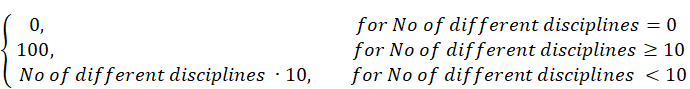
(104)
The level of engagement (LE) metric assesses the level of collaboration among the professionals/highly skilled workers from the different disciplines included in a project. Relevant information on the level of collaboration can be directly retrieved by results of existing interviews (if any) with the professionals or by specific documents/reports of meetings/workshops during the project design phase providing data on the degree of interaction among the professionals/highly skilled workers of the project team. LE score is evaluated via a 5‑point Likert scale (Joshi et al., 2015), thus resulting into five fixed values depending on the quality of the level of collaboration towards a full engagement among the professionals/highly skilled workers from the different disciplines involved in the project, ranging from very poor to very strong, according to the rationale in Table 42.
Table 42. Level of engagement metric score.
Sub-metric | Score |
Select single value from the sub-metrics below: | |
Each discipline worked without interaction (i.e. very poor engagement) | 0.2 |
Professionals of some disciplines expressed opinions (i.e. poor engagement) | 0.4 |
Professionals of all disciplines expressed opinions and provided reports (i.e. acceptable engagement) | 0.6 |
Organisation of workshops for the interaction of the professionals of all disciplines without necessarily reaching a consensus (i.e. strong engagement) | 0.8 |
Engagement among the professionals through workshops and final agreement and consensus (i.e. very strong engagement) | 1 |
| Metric score = one of the five sub-metric scores | LE = 0.2 or 0.4 or 0.6 or 0.8 or 1 |
Source: JRC.
The indicative thresholds to associate the S.7.2 indicator score to the indicator performance class are provided in Figure 39. The Low, Acceptable, Good, and Excellent performance classes for the S.7.2 indicator correspond to the following ranges of S.7.2 scores, i.e. 0 ≤ S.7.2 < 10, 10 ≤ S.7.2 < 40, 40 ≤ S.7.2 < 80, and 80 ≤ S.7.2 ≤ 100, respectively. While the indicator thresholds and performance classes are not directly applied in the evaluation of KPI and dimension scores and performance classes, they are included here to assist users in determining appropriate performance levels for specific project aspects and to offer clear guidance on their improvement.
Figure 39. S.7.2 indicative performance classes and thresholds.

Source: JRC.
3.10.4 Gross value added to local economy from new business creation (S.7.3)
The gross value added to local economy from new business creation (S.7.3) indicator evaluates the ability of a public entity to stimulate the local economy throughprojects in line with the NEB vision by ensuring that the project development attracts inward investment, creates jobs, and complements and enhances existing economic activities. S.7.3 indicator is fully aligned to the SDG 8 (UN, Resolution 2015), which promotes inclusive and sustainable economic growth, full and productive employment, and decent work for all.
The extent of a job creation or destruction can significantly shape the social acceptance and desirability of different interventions related to NEB, also leading to social mobilisation to support or oppose future decarbonisation activities and green transition pathways. Past studies related the direct and/or indirect contribution of green transition activities and investments in creating possible new jobs. According to Renner at al. (2008), greening the building industry in the EU and the United States would create al least 2million jobs, which increase to 3.5 million considering a scenario of 75 % CO2-emission reduction in the residential building sector by 2030. A 2012 analysis (Næss-Schmidt et al., 2012) estimated that the energy renovation of the European building stock could have led to 0.75–1.5 million new jobs per year if undertaking annual investments of EUR 40 billion until 2020. Similarly, every EUR 1 million investment in the energy efficiency of buildings may correspond on average to 19 new jobs (Jassen and Staniaszek, 2012). Recent studies further stress the link of the possible growth in employment in the EU to the investment needed to meet the green transition goal, leading to the increase of ‘green jobs’[1]. Indeed, the green transition will profoundly impact Europe's labour markets: it was estimated that the more ambitious climate target to meet a 55 % reduction in GHG emissions in the EU by 2030, compared with 1990 could lead to a net increase in jobs of up to 884 000 by 2030 (Asikainen et al., 2021) Similarly, a recent study (Sovacool et al., 2023) analysed the way one aspect of green transition, i.e. making buildings dependent on self-produced renewable energy, contributes to employment growth in the energy industry, not exploring aggregate job creation within regions/nations or globally, but considering a micro-scale approach assessing job creation at level of individual residential and non-residential buildings equipped with three low-carbon technologies, namely solar PV, batteries for energy storage, heat pumps for the electrification of heating and cooling. Specifically, results pointed out that the largest share of job years derives from construction and installation of the three technologies.
In this context, it is crucial to demonstrate that the implementation of projects in line with the NEB vision may lead to the creation of new green jobs, new businesses, and/orthe improvement of existing working conditions (e.g. higher-paying employment) for a two-fold reason: (i) attract investment and funding for the implementation of a specific project and similar future projects, and (ii) foster public support for the projects. Indeed, institutional and private investors are increasingly interested in projects that can generate positive social and environmental impacts, and financial returns, as well as citizens are more likely to support projects that clearly benefit their community.
The implementation of a project through its corresponding investment can generate three types of job effects to be estimated: (i) direct job effects concern the creation of new jobs, more likely at local level, directly through increased demand of employment for the design and implementation (e.g. via construction, operations, maintenance) of the project and related services, (ii) indirect job effects arise in supplier industries of the sustainable economy providing intermediate goods for the project (e.g. green building components, renewable energy technologies, clean mobility, social services, etc.), and (iii) induced job effects occur as savings from the project benefits (e.g. reduction of energy consumption) and wage incomes are spent in goods and services generating demand in additional industries. Employment aspects related to salaries and business income may be complemented by introducing weighting parameters to relate them to the local living wage, as Member States in the EU and even regions within the same Member State may have very different living costs.
Based on this overview, the following three assumptions are considered to evaluate the S.7.1 score:
- Every investment of EUR 1 million in projects for the energy renovation of existing buildings can generate 19 new permanent jobs in the building sector (although not at the local level). However, an amount up to EUR 6 million may be needed to create an additional job for a person living in the target area (Næss-Schmidt et al., 2012).
- In 2021, the annual average full-time adjusted salary per employee in the EU was estimated equal to EUR 33500 (Eurostat, 2022).
- A project in line with the NEB vision creates economic value and new jobs with a contract of 3 years per job. In the context of the S.7.1 score evaluation, if a contract is less than 3 years per job, then it is projected to be 3 years; for example, if a contract refers to 1 job for 1 year, then it is 0.33 jobs for 3 years.
- According to assumption (2) and (3), the monetary value (MV) of one job with a 3-year contract is calculated according to Equation (105) and the result is rounded to a value equal to EUR 100000; consequentially, a monetary value of EUR 1 million corresponds to a maximum number of local jobs with a 3‑year contract equal to 10.

(105)
S.7.3 score is calculated according to Equation (106) as the ratio of the monetary value of the jobs created by the project to the total monetary budget of the project; multiplied by 100, so that the score can be expressed as a dimensionless value that varies between 0 and 100.
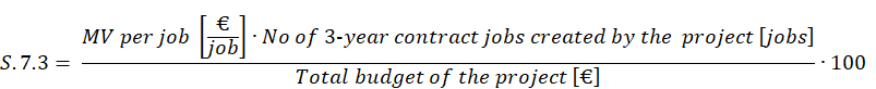
(106)
The indicative thresholds to associate the indicator score to the indicator performance class are provided in Figure 40. The Low, Acceptable, Good, and Excellent performance classes for the S.7.3 indicator correspond to the following ranges of S.7.3 scores, i.e. 0 ≤ S.7.3 < 10, 10 ≤ S.7.3 < 40, 40 ≤ S.7.3 < 80, and 80 ≤ S.7.3 ≤ 100, respectively. While the indicator thresholds and performance classes are not directly applied in the evaluation of KPI and dimension scores and performance classes, they are included here to assist users in determining appropriate performance levels for specific project aspects and to offer clear guidance on their improvement.
Figure 40. S.7.3 indicative performance classes and thresholds

Source: JRC.
[1] Green jobs: International Labour Organization & United Nations (2016); https://www.ilo.org/resource/article/what-green-job
3.10.5 Example (S.7)
An investment of EUR 15 million is provided by public entities for a renovation project of a brownfield urban site into an area with residential buildings and green spaces. A total number of 50 members constitutes the team of professionals/highly skilled workers involved in the project design and the number of different disciplines within the team equals to 5. Moreover, the level of collaboration among the team members of the different disciplines during the design of the intervention is based on relevant information directly reported by the team members. The neighbourhood scale project was in open consultation with the local inhabitants, and one workshop was performed to present the project. The investment also creates jobs in the construction, remediation, and landscaping sectors. The construction sector implies energy efficiency and renewable energy skills, leading to jobs in retrofits, installations, and maintenance. Moreover, a new public transportation line is added, potentially creating one additional job at least in operation phase. The new green space and parks can also create two jobs in maintenance and management of socio-cultural-motorial activities. In addition to the benefits provided by the creation of these direct jobs, the project can lead to the creation of indirect jobs by supporting local businesses and attracting new businesses to the area. Assuming that an economic analysis based on local data shows the lack of restaurants in the designated area of the project, the regenerated neighbourhood may attract restaurants, cafes, and grocery shops to satisfy the needs of new residents, thus creating new indirect jobs related to food service and hospitality. Specifically, 12 new direct jobs with a 3-year contract each have been created at local level.
The evaluation of the S.7 S.7 KPI to achieve the possible greening of the public sector depends on the scores of S.7.1, S.7.2, and S.7.3 indicators.
S.7.1 score is estimated according to the metrics in Table 41. S.7.1 score is based on the application of the SROI anlysis to the project, thus leading two out of four metrics in the form of consecutive statements to be satisfied, as reported in Table 43. Indeed, stakeholders, namely the residents of the neighbourhood area, who also participate to the workshop to present the project, were involved into the project analysis; whereas changes resulting from the project were not expressed in monetary values and a forecast SROI was not performed. The S.7.1 score, resulting into a value equal to 50, corresponds to the indicative Acceptable performance class (Figure 38).
Table 43. Example of S.7.1 evaluation.
| Metric | Score |
| The social return on investment (SROI) analysis is applied to the project. | Check next metrics. |
| Stakeholders have been involved in the project to determine the outcomes of the project. | 20 |
| Workshops have also been performed to understand the changes experienced by the stakeholders. | 50 |
| Indicator score = one of the potential five metric scores | S.7.1 = 50 |
Source: JRC
The evaluation of S.7.2 score relies on the following two metrics: (i) number of disciplines (ND), and (ii) level of engangement (LE).
The number of disciplines (ND) metric is evaluated by using Equation (104) according to the third condition indicated in that equation, as the number of different disciplines equals 5. Hence, ND score is estimated equal to 50 (Equation (107)), as follows:
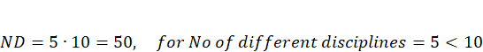 |
(107)
The level of engagement (LE) metric is estimated according to the sub-metrics in Table 42, leading to an acceptable quality of the engagement among professionals/highly skilled workers of all disciplines considered within the project, as they expressed opinions and provided reports during the project design phase.Thus, the LE score equals to 0.6.
From Equation (103), the score of the S.7.2 indicator is estimated equal to 30 (Equation (108)). Accordingly, the S.7.3 score is associated to the indicative Acceptable performance class (Figure 39).
 |
(108)
The S.7.3 score is estimated by using Equation (106), considering that the monetary value per job is equal to EUR 100 000 and the total budget of the project corresponds to the investment of EUR 15 million. Hence, S.7.3 score is estimated equal to 8 (Equation (108)), which corresponds to an indicative Low performance class for S.7.3 indicator (Figure 40).
 |
(109)
Having evaluated the scores of S.7.1, S.7.2, and S.7.3 indicators, S.7 is evaluated by using Equation (102), resulting into a score equal to 23 that corresponds to the Acceptable performance class (Figure 37), as reported in Table 44.
Table 44. Example of S.7 evaluation
| Indicator | S.7.1 | S.7.2 | S.7.3 |
| Indicator score | 50 | 30 | 8 |
| Indicator performance class (indicative) 1 | (Acceptable) | (Acceptable) | (Low) |
| S.7 score | 0.2 • 50 + 0.3 • 30 + 0.5 • 8 = 23 | ||
| S.7 performance class | Acceptable | ||
| S.7 performance class score (PCSS.7) | 45 | ||
1 Transformation of the indicator score to an indicator performance class is indicative and not required by the self-assessment method to estimate KPI and dimension scores and performance classes.
3.11 Achieve the best possible greening of the private and financial sector in terms of its economic involvement in the sustainability of the built environment (S.8)
3.11.1 Description and assessment
Achieve the possible greening of the private and financial sector in terms of its economic involvement (S.8) KPI is assessed through the following two indicators:
- Green financial tools (S.8.1).
- Compliance with ESG standards and European Sustainability Reporting Standards (ESRS) for green transition investments from private companies (S.8.2).
In the general case when both indicators are considered, S.8 score is evaluated according to Equation (110).
(110)
Specifically, S.8.2 indicator is evaluated only when the European Sustainability Reporting Standards (ESRS) are mandatory for use by at least one private company (involved in the project) that is obliged by the Corporate Sustainability Reporting Directive (CSRD) (Directive, 2022) to report specific sustainability information on their performance. Accordingly, if no private company involved in the project is obliged by the CSRD (Directive, 2022) to use the ESRS to fulfill sustainability reporting obligations, S.8.2 is omitted and S.8 score is evaluated according to Equation (111).
(111)
S.8 thresholds to associate the KPI score to the performance class adopted in the self-assessment method are provided in Figure 41. The Low, Acceptable, Good, and Excellent performance classes of S.8 correspond to the following ranges of S.8 scores, i.e. 0 ≤ S.8 < 15, 15 ≤ S.8 < 40, 40 ≤ S.8 < 80, and 80 ≤ S.8 ≤ 100, respectively.
Figure 41. S.8 performance classes and thresholds

Source: JRC.
S.8 and its two associated indicators can be applied at building, neighbourhood and urban scale, including both newbuild and renovation projects with both residential and non-residential use.
3.11.2 Green financial tools (S.8.1)
The green financial tools (S.8.1) indicator refers to special terms, incentives, or benefits for a project that traditional financial instruments do not provide. The indicator recognises and measures the extent of the use of private green financial tools over the total private funding used for a project, helping in understanding the financial health and strategy of the project, while mainstreaming the green finance. The more a NEB project adopts and showcases the use of green financial tools, the more normalized these tools become in the industry and will assist in the greening of the private and financial sector. Additionally, S.8.1 indicator through the specific focus on green financing, can spur further innovation in sustainable technologies and practices, as there's a clear financial incentive to adopt them.
S.8.1 score is evaluated as the ratio of private green funding tools (i.e. examples of green financial instruments are defined in Table 3) used for a project to the total private funding, multiplied by 100, according to Equation (112).

(112)
S.8.1 indicative thresholds to associate the indicator score to the corresponding indicator performance class are provided in Figure 42. The Low, Acceptable, Good, and Excellent performance classes of S.8.1 correspond to the following ranges of S.8.1 scores, i.e. 0 ≤ S.8.1 < 15, 15 ≤ S.8.1 < 40, 40 ≤ S.8.1 < 80, and 80 ≤ S.8.1 ≤ 100, respectively. While these thresholds and performance classes are not directly applied in the evaluation of KPI and dimension scores and performance classes, they are included here to assist users in determining appropriate performance levels for specific project aspects and to offer clear guidance on their improvement.
Figure 42. S.8.1 indicative performance classes and thresholds

Source: JRC.
3.11.3 Compliance with ESG standards and European Sustainability Reporting Standards for green transition investments from private companies (S.8.2)
The compliance with ESG standards and ESRS and Green Transition Investments from private companies (S.8.2) indicator assesses the green transition investments in a project compliant with the NEB vison. The S.8.2 indicator is evaluated only if at least one of the private companies involved in the project is obliged by the CSRD to follow the requirements for their sustainability performance reporting, according to the European Sustainability Reporting Standards (ESRS). The ESRS (Baumüller and Grbenic, 2021; Giner and Luque-Vílchez, 2022) targets to enhance the scope and quality of corporate sustainability reporting while promoting sustainable development through increased transparency. Stakeholders, particularly investors, other businesses, and society at large, should have access to better insights into companies' business practices. The European Sustainability Reporting Standards (ESRS) require companies to provide detailed information about their sustainability performance, sometimes extending all the way to the supply chain and product life cycle.
This shift demands more robust data management and the refinement of existing reporting structures and processes, particularly since the Corporate Sustainability Reporting Directive (CSRD) mandates an electronic format for sustainability data. Notably, companies governed by the CSRD are not required to produce a separate sustainability report compliant with the ESRS; rather, sustainability information is integrated into the groups' annual report. Importantly, this non-financial information regarding sustainability is also subject to external audit requirements. Companies must be prepared to explain how specific environmental, social, and governance data and key performance indicators are collected.
Overall, the ESRS enhances the quality and comparability of reporting content. However, the implications of the ESRS extend beyond mere reporting mandates. These standards also require companies to disclose improvements in their sustainability performance and advancements in sustainability management. Ultimately, these requirements aim to hasten the transition toward a sustainable economy. The new CSRD standards are integral to the EU’s strategic plan to achieve climate neutrality by 2050 and to foster a sustainable economic framework. Alongside the ESRS and the EU Taxonomy Regulation, the Corporate Sustainability Due Diligence Directive and various other EU initiatives play critical roles in the march toward the EU Green Deal.
Specifically, the CSRD identifies the companies that are required to publish annual report on their social and environmental performance, according to the ESRS, along with the fiscal year the corresponding companies have to apply the new rules for the first time, as follows (Directive, 2022/2464):
- From fiscal year 2024, for reports published in2025: companies that are already subject to a reporting obligation under the Non-Financial Reporting Directive (Directive, 2014/95/EU).
- From fiscal year 2025, for reports published in 2026: all other large corporations with an annual average of 250 employees or more, total assets of 25 million euros or EUR 50 million in sales. Two of these three criteria must be met for a company to fall within the scope of the CSRD.
- From fiscal year 2026, for reports published in 2027: listed SMEs, small and non-complex credit institutions, and captive insurance companies.
For reports published in 2029, from fiscal year 2028: third-country companies with subsidiaries or branches in the EU that generate a net turnover of more than EUR 150 million in the Union for two consecutive financial years.
The S.8.2 indicator is evaluated only if the following statement is satisfied for at least one of the private companies involved in a project: The private company involved in the project is under the scope of the CSRD to mandatory fulfill sustainability reporting obligations, according to ESRS. If this statement is satisfied, the S.8.2 indicator is evaluated through the two following metrics:
- Total own funding investments (Total OFI).
- Total green investments (Total GI).
The S.8.2 score is estimated as the ratio of the Total GI metric to the Total OFI metric, multiplied by 100 to provide a dimensionless score that varies between 0 and 100, according to Equation (113).
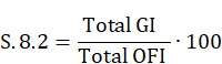
(113)
The Total GI metric is estimated as the sum of the green investment of the i-th company involved in the project, according to Equation (114), in which N is the total number of the private companies involved in the project.
(114)
The Total OFI metric is estimated as the sum of the own funding investment of the i-th company involved in the project, according to Equation (115), in which N is the total number of private companies involved in the project.
(115)
The S.8.2 thresholds to associate the indicator score to its corresponding performance classare provided in
Figure 43. The Low, Acceptable, Good, and Excellent performance classes of S.8.2 correspond to the following ranges of S.8.2 scores, i.e. 0 ≤ S.8.2 < 15, 15 ≤ S.8.2 < 40, 40 ≤ S.8.2 < 80, and 80 ≤ S.8.2 ≤ 100, respectively. While these thresholds and performance classes are not directly applied in the evaluation of KPI and dimension scores and performance classes, they are included here to assist users in determining appropriate performance levels for specific project aspects and to offer clear guidance on their improvement.
Figure 43. S.8.2 indicative performance classes and thresholds

Source: JRC.
3.11.4 Example (S.8)
An investment of EUR 15 million in the redevelopment of a brownfield urban site into residential buildings and green spaces is considered. The consortium of investors includes three private companies, specifically consisting of two private manufacturers and one consultancy private company, hereinafter indicated as company 1, company 2, and company 3. A private green funding equal to EUR 3 million is ensured via green bonds and other green financing tools for the project development., whereas the total private funding for the project corresponds to50 % of the investment, thus being equal to EUR 7.5 million.. Company 1, which is one out of the two private manufacturers has invested own funds equal to EUR 500 000 in the project and invested in green transition with 100K€ in photovoltaics in their office building. Company 2, corresponding to the other private manufacturer, has invested EUR 1 million in a new property with its own funds. Company 3 that refers to the consultancy company has invested EUR 200 000, which represents the 20 % of its own funding scheme, in a circular economy start-up company. For all three companies, at the time of the assessment the ESRS is mandatory.
The evaluation of S.8 KPI depends on the evaluation of S.8.1 and S.8.2 indicator scores, as the ESRS apply mandatory to.
S.8.1 score is evaluated by using Equation (54), resulting into a value equal to 40 (Equation (116)). Accordingly, the S.8.1 score is associated to the indicative Good performance class (Figure 42).
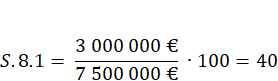 |
(116)
S.8.2 score relies on the rationale that the following statement needs to be satisfied: the private company involved in the project is under the scope of the CSRD to mandatory fulfill sustainability reporting obligations, according to ESRS. All the three private companies involved in the project satisfy the statement, thus the S.8.2 score can be evaluated based on the two following metrics: (i) total own funding investiment (Total OFI), and (ii) total green investment (Total GI).
The total OFI metric is estimated by using Equation (115), considering the OFI of each of the three companies, as follows (Equation (117)).
 |
(117)
The total GI metric is estimated by using Equation (114), considering the GI of the company 1 and 3 (company 2 has not invested in green projects), as follows (Equation (118)).
(118)
The evaluation of the score of S.8.2 indicator is based on Equation (113), resulting into a score equal to 12, as follows (Equation (119)). S.8.2 score corresponds to the indicative Low performance class.
 |
(119)
Having evaluated the scores of S.8.1 and S.8.2 indicators, S.8 is calculated by using Equation (111), resulting into a score equal to 26 that corresponds to the Acceptable performance class (Figure 41), as summarised in Table 45.
Table 45. Example of S.8 evaluation
| Indicator | S.8.1 | S.8.2 |
| Indicator score | 40 | 12 |
| Indicator performance class (indicative) 1 | (Good) | (Low) |
| S.8 score | 0.5 • 40 + 0.5 • 12 = 26 | |
| S.8 performance class | Low | |
| S.8 performance class score (PCSS.8) | 25 | |
1 Transformation of the indicator score to an indicator performance class is indicative and not required by the self-assessment method to estimate KPI and dimension scores and performance classes..
Source: JRC.
3.12 Promote circular economy in the built environment (S.9)
3.12.1 Description and assessment
Promote circular economy in the built environment (S.9) KPI aims to point out the rate of using secondary and biobased materials in the construction industry, contributing to close the circularity loop of materials through the use of less impactful and more regenerative materials.
S.9 is evaluated through one main indicator, as follows:
- Secondary, bio-based, recycled materials (S.9.1).
S.9 score is calculated according to Equation (120), thus corresponding to S.9.1 score.
(120)
The S.9 thresholds adopted in the self-assessement method to associate the KPI score to the KPI performance classare provided in Figure 44. The Low, Acceptable, Good, and Excellent performance classes of S.9 correspond to the following ranges of S.9 scores, i.e. 0 ≤ S.9 < 10, 10 ≤ S.9 < 40, 40 ≤ S.9 < 80, and 80 ≤ S.9 ≤ 100, respectively.
Figure 44. S.9 performance classes and thresholds.

Source: JRC.
S.9 and its associated indicator can be applied at all the three spatial scales of a project (i.e. building, neighbourhood, and urban), including both newbuild and renovation projects with residential and non-residential use.
3.12.2 Secondary, bio-based, recycled material (S.9.1)
Secondary, bio-based, recycled material (S.9.1) is based on the circularity indicator proposed into the recent standard ISO 59020 (ISO, 2024c), as well as on the material circularity indicator within the ‘Circular Transition Indicator’ framework developed by the World Business Council for Sustainable Development (WBCSD, 2022b). Accordingly, the S.9.1 indicator measures the circularity of materials within a project by considering the share of secondary, bio-based and recycled materials in relation to the total amount of materials used in a project, thus S.9.1 is evaluated through the following metric:
- Circularity of material (CM).
S.9.1 score is estimated as the product of the CM metric by both a constant k (i.e. k = 5) and 100, so that the indicator score is expressed as a dimensionless value that varies between 0 and 100, according to Equation (121).
(121)
The Circularity of material (CM) score is calculated as the as the ratio of the mass or cost of secondary, bio-based and recycled materials used in a building/neighbourhood/urban project to the total mass of the total amount of materials used in the project, expressed as a percentage, according to Equation (122).

(122)
In the Equation (121), the value of the constant k is based on the EU circular material use rate (CMUR) target by 2030. Specifically, the CMUR, which refers to the share of the total amount of material used in the EU-27 coming from recycled waste materials, is quite low with the recycled material accounting for 11.5 % of total material used in 2022 (Eurostat, 2023c). The 2022 figure should increase to 23.2 % by 2030 to meet the target of doubling the CMUR compared to the 2020 rate (COM 98/2020). Based on this projection, the S.9.1 score evaluation relies on the assumption that the maximum value of CM (CMmax) is equal to 20 %, thus CM score ranges between 0 % and 20 %. According to this assumption, CMmax needs to be multiplied by a constant that results into a value equal to 5 to achieve the S.9.1 maximum score equal to 100 (i.e. S.9.1 = CMmax ∙ k ∙100 → 100 = 20 ∙ k → k =5). In the case of the CM score being higher than 20 %, the S.9.1 score cannot exceed 100.
The indicative thresholds to associate the S.9.1 indicator score to the indicator performance classes are provided in Figure 45 for sake of completeness since the S.9.1 thresholds correspond to the S.9 ones, as expected. The Low, Acceptable, Good, and Excellent performance classes for the S.9.1 indicator correspond to the following ranges of S.9.1 scores, i.e. 0 ≤ S.9.1 < 10, 10 ≤ S.9.1 < 40, 40 ≤ S.9.1 < 80, and 80 ≤ S.9.1 ≤ 100, respectively. While the indicator thresholds and performance classes are not directly applied in the evaluation of KPI and dimension scores and performance classes, they are included here to assist users in determining appropriate performance levels for specific project aspects and to offer clear guidance on their improvement.
Figure 45. S.9.1 indicative performance classes and thresholds

Source: JRC.
3.12.3 Example (S.9)
A building with a total floor area equal to 4000 m2 and its surrounding area equal to 5 acres is refurbished following the NEB concept. A circular economy strategy is adopted by re-using all secondary concrete and stone materials to build the courtyard and the pedestrian paths around the building. The mass of secondary, bio-based, recycled materials used in the project is equal to 500 tons. The total mass of materials used in the project is estimated to be 12500 tons.
The evaluation of S.9 depends on S.9.1 score, which relies on the CM metric. The CM score is calculated by using the Equation (122), thus estimating that 4 % of the total amount of material used in the project comes from secondary, bio-based, recycled materials, as follows (Equation (123)):
 |
(123)
Accordingly, the B.9.1 score is evaluated from Equation (121), as follows (Equation (124)):
 |
(124)
Having evaluated the S.9.1 score, the S.9 score is calculated by using Equation (120), resulting into a value equal to 20, thus corresponding to the Acceptable performance class (Figure 44), as reported in Table 46.
Table 46. Example of S.9 evaluation.
| Indicator | S.9.1 |
| Indicator score | 20 |
| Indicator performance class (indicative) | (Acceptable)1 |
| S.9 score | = 1 ∙ 20 = 20 |
| S.9 performance class | Acceptable |
| S.9 performance class score (PCSS.9) | 45 |
1 Transformation of the indicator score to an indicator performance class is indicative and not required by the self-assessment method to estimate KPI and dimension scores and performance classes.
Source: JRC.